Field Definitions
This page defines the field quantities TI-Toolbox computes and reports: the TI envelope and its directional variants, the carrier fields, and the focality ratios built from them. The Analyzer, the Simulator and the optimizers link here for the maths. Each section opens with the idea in words and one key equation; derivations, accuracy and edge cases sit in the collapsible Details blocks.
Each field has a saved name, used in files, configs and scripts, and a display label the app, the Viewer and these pages show:
| Saved name | Shown as | Units | What it is |
|---|---|---|---|
TI_max (mTI_max for mTI) |
\(TI_{max}\) (\(mTI_{max}\)) | V/m | envelope modulation depth, maximised over direction |
TI_normal |
\(TI_{normal}\) | V/m | the envelope along the cortical surface normal |
TI_avg |
\(TI_{avg}\) | V/m | the envelope averaged over direction |
hf_peak |
\(HF_{peak}\) | V/m | peak (zero-to-peak) carrier field |
hf_rms |
\(HF_{rms}\) | V/m | RMS carrier field over time |
hf_power_density |
\(p_{HF}\) | W/m³ | absorbed (Joule) power density of the carriers |
Notation. At one point (mesh element or voxel):
- \(\mathbf{E}_1, \dots, \mathbf{E}_N\): the channels’ field amplitudes (V/m); for two channels, \(\mathbf{E}_1\) and \(\mathbf{E}_2\).
- \(\hat{\mathbf{n}}\): a unit direction; \(a = \mathbf{E}_1 \cdot \hat{\mathbf{n}}\) and \(b = \mathbf{E}_2 \cdot \hat{\mathbf{n}}\) are the channels along it.
- \(K\): the number of beating pairs; \(\Delta f\) their common beat frequency.
- \(E_{\mathrm{AM}}(\hat{\mathbf{n}})\): the envelope amplitude along \(\hat{\mathbf{n}}\).
Field quantities
A channel is one electrode pair driven by one current source at its own kHz carrier frequency. Two channels whose carrier frequencies differ by a small \(\Delta f\) form a beating pair and beat at \(\Delta f\). Standard TI is one beating pair: two channels at slightly different carrier frequencies (4 electrodes, for example 2.000 and 2.010 kHz). Multipolar TI (mTI) uses \(2K\) channels in \(K\) beating pairs, all beating at a common \(\Delta f\) (8 electrodes for \(K = 2\), for example 2.000/2.010 and 4.000/4.010 kHz).
A kHz field alone does not modulate neurons. What matters is the amplitude of the slow beat where the channels’ fields overlap (Grossman et al. 2017). Every statistic the Analyzer reports summarises that amplitude, or one of the carrier fields, over space.
TI_max stores at every mesh element or voxel.
Two channels: the envelope amplitude
Along a direction \(\hat{\mathbf{n}}\) the two channels are sinusoids of amplitude \(a\) and \(b\). Their sum swings between \(\lvert a \rvert + \lvert b \rvert\) and \(\bigl\lvert \lvert a \rvert - \lvert b \rvert \bigr\rvert\) once per beat, so the envelope amplitude along \(\hat{\mathbf{n}}\) is
\[E_{\mathrm{AM}}(\hat{\mathbf{n}}) = \Bigl\lvert \, \lvert (\mathbf{E}_1 + \mathbf{E}_2) \cdot \hat{\mathbf{n}} \rvert - \lvert (\mathbf{E}_1 - \mathbf{E}_2) \cdot \hat{\mathbf{n}} \rvert \, \Bigr\rvert = 2 \min\bigl( \lvert a \rvert, \lvert b \rvert \bigr)\]TI_max (V/m) is its maximum over all directions, \(E_{\mathrm{AM}}^{\max}\), which has a closed form. Label the channels so that \(\lVert \mathbf{E}_1 \rVert \ge \lVert \mathbf{E}_2 \rVert\), and flip the sign of \(\mathbf{E}_2\) if needed so that the angle \(\alpha\) between the fields is at most 90°. Then
Details: reading the condition, names in the literature, implementation
The condition is easiest to read along \(\mathbf{E}_2\) itself, where the projections are \(\lVert \mathbf{E}_1 \rVert \cos\alpha\) and \(\lVert \mathbf{E}_2 \rVert\): when the first is the larger, that direction reaches the full \(2 \lVert \mathbf{E}_2 \rVert\). Otherwise the maximum lies in the plane of the two fields, perpendicular to \(\mathbf{E}_1 - \mathbf{E}_2\), and is smaller.
Both formulas are from Grossman et al. 2017 (Cell 169:1029, STAR Methods), who call \(E_{\mathrm{AM}}\) the envelope modulation amplitude. SimNIBS calls \(E_{\mathrm{AM}}^{\max}\) “TImax”, Hirata et al. 2024 call it the electric field envelope (EFE) amplitude, and this toolbox stores it as TI_max (V/m). The code and some figures call \(E_{\mathrm{AM}}\) the modulation depth (MD). tit.calc.envelope_max evaluates an equivalent form that needs no relabelling or sign flip (Hirata et al. 2024, Computers in Biology and Medicine 178:108697, Eq. 2); it agrees with SimNIBS’s TI_utils.get_maxTI to rounding.
Direction: TI_max, TI_normal, TI_avg, tangential
The envelope fields differ only in which directions \(\hat{\mathbf{n}}\) they use:
| Field | Direction | Meaning | tit.calc function |
|---|---|---|---|
TI_max (mTI_max for mTI) |
the maximum over all \(\hat{\mathbf{n}}\) | the strongest modulation a neuron at that point could see, whatever its orientation; the default output and the default score of every optimizer | envelope_max(fields) |
TI_normal (mesh only) |
the normal of the central (mid-thickness) grey-matter surface at each node | the modulation along the axis of pyramidal-cell apical dendrites; written by every simulation that has a beat | envelope(fields, normals) |
TI_avg (optional) |
the mean over all \(\hat{\mathbf{n}}\) | what a randomly oriented neuron sees on average | envelope_mean(fields) |
tangential TI (flex-search dir_TI_tangential) |
the maximum over the \(\hat{\mathbf{n}}\) in the surface plane, perpendicular to the normal | the strongest modulation along the cortical sheet | envelope_max(fields, perpendicular_to=normals) |
By definition none of TI_normal, TI_avg and the tangential maximum exceeds TI_max, and TI_normal collapses where the field runs tangential to the cortex. For two channels, \(\mathrm{TI\_normal} = 2 \min\bigl( \lvert \mathbf{E}_1 \cdot \hat{\mathbf{n}} \rvert, \lvert \mathbf{E}_2 \cdot \hat{\mathbf{n}} \rvert \bigr)\): each channel’s field is reduced to its normal component first, and then the beat amplitude of those two components is taken.
For two channels the mean over directions has a closed form:
\[\mathrm{TI\_avg} = \lVert \mathbf{E}_1 \rVert + \lVert \mathbf{E}_2 \rVert - \tfrac{1}{2}\bigl( \lVert \mathbf{E}_1 + \mathbf{E}_2 \rVert + \lVert \mathbf{E}_1 - \mathbf{E}_2 \rVert \bigr)\]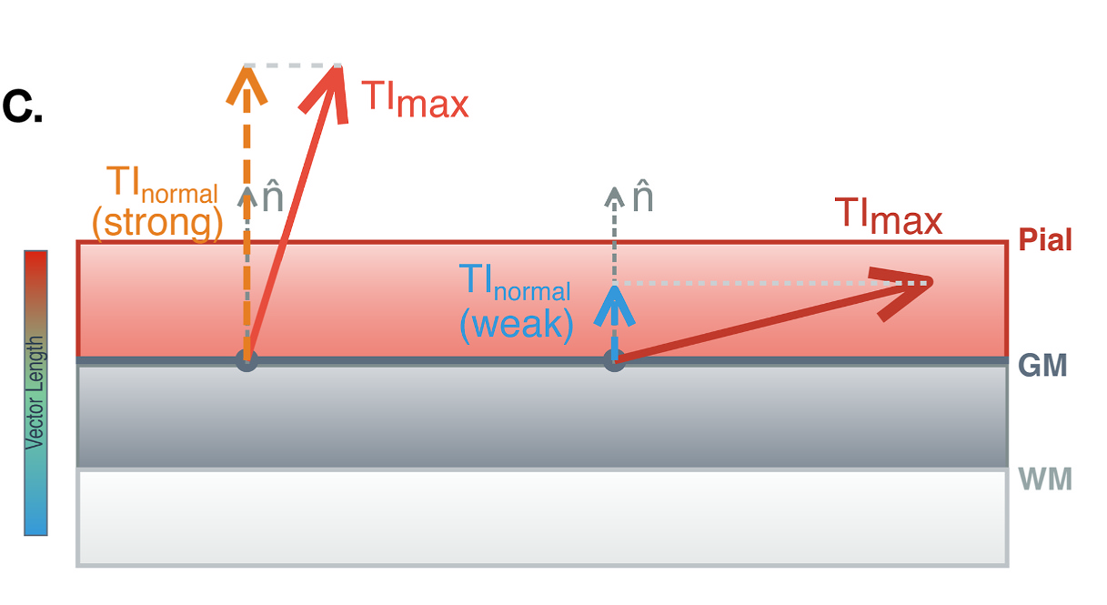
TI_normal is the envelope amplitude along the local surface normal \(\hat{\mathbf{n}}\). Where the strongest modulation runs along \(\hat{\mathbf{n}}\) (left) the two values are close; where it runs tangential to the cortex (right) TI_normal is small although TI_max is unchanged. The dashed drop lines are schematic: TI_normal is the envelope evaluated along \(\hat{\mathbf{n}}\), not the projection of the TI_max vector onto \(\hat{\mathbf{n}}\). Figure 4C from Haber et al. 2026.
Details: why TI_normal is not a projection, the TI_avg derivation, the tit.calc functions
TI_normal is not the normal component of the TI_max vector, because the envelope is not linear in the fields. With \(\mathbf{E}_1 = \hat{\mathbf{x}}\), \(\mathbf{E}_2 = \hat{\mathbf{y}}\) and the normal along \(\hat{\mathbf{x}}\), the TI_max vector \((1, 1, 0)\) projects to 1, but TI_normal is 0, because the second channel has no normal component to beat with. For the same reason the tangential maximum is not \(\sqrt{\mathrm{TI\_max}^2 - \mathrm{TI\_normal}^2}\): it is the envelope maximised over the in-plane directions, which equals TI_max of the two fields projected onto the surface plane.
The TI_avg closed form follows because \(E_{\mathrm{AM}} = 2\lvert a \rvert + 2\lvert b \rvert - \lvert a + b \rvert - \lvert a - b \rvert\) and the mean of \(\lvert \mathbf{v} \cdot \hat{\mathbf{n}} \rvert\) over the sphere is \(\lVert \mathbf{v} \rVert / 2\).
tit.calc has five functions: envelope, envelope_max and envelope_mean for the envelope, and hf_peak and hf_power for the carriers (Carrier fields). The envelope functions take fields = [E_1, E_2, ..., E_2K], one (N, 3) array per channel, with each two consecutive channels forming a beating pair. envelope_max(fields, return_direction=True) also returns the unit direction of the maximum; TI_max times that direction is the TI vector the Blender export draws. Every simulation, ex-search and mex-search computes its envelope fields with these functions.
More beating pairs: multipolar TI (mTI)
With \(K\) beating pairs the pairs’ power envelopes add, not their amplitudes. The envelope amplitude along \(\hat{\mathbf{n}}\) is
\[E_{\mathrm{AM}}(\hat{\mathbf{n}}) = \Bigl\lvert \, \lVert \mathbf{S} \hat{\mathbf{n}} \rVert - \lVert \mathbf{D} \hat{\mathbf{n}} \rVert \, \Bigr\rvert = \frac{4 \, \bigl\lvert \sum_{k} a_k b_k \bigr\rvert}{\lVert \mathbf{S} \hat{\mathbf{n}} \rVert + \lVert \mathbf{D} \hat{\mathbf{n}} \rVert}\]where
- pair \(k\)’s two channels are \(\mathbf{E}_{2k-1}\) and \(\mathbf{E}_{2k}\) (carriers \(f_k\) and \(f_k + \Delta f\)), the order
tit.calcexpects, and \(a_k = \mathbf{E}_{2k-1} \cdot \hat{\mathbf{n}}\), \(b_k = \mathbf{E}_{2k} \cdot \hat{\mathbf{n}}\); - \(\mathbf{S}\) and \(\mathbf{D}\) are the \(K \times 3\) matrices whose rows are \(\mathbf{E}_{2k-1} + \mathbf{E}_{2k}\) and \(\mathbf{E}_{2k-1} - \mathbf{E}_{2k}\).
The right-hand form subtracts no near-equal numbers and is the one the code evaluates. TI_max for mTI is the maximum of \(E_{\mathrm{AM}}(\hat{\mathbf{n}})\) over directions, as for two channels; mTI meshes name it mTI_max. TI_normal is the same expression at the surface normal, and TI_avg its mean over the sphere.
Details: derivation, assumptions, unpaired channels
Squaring the summed signal and low-pass filtering it removes every kHz term and leaves the power envelope
\[p(t) = P + Q \cos(2\pi \Delta f \, t), \qquad P = \frac{1}{2} \sum_{k=1}^{K} \left( a_k^2 + b_k^2 \right), \qquad Q = \sum_{k=1}^{K} a_k b_k\]\(P\) is the mean carrier power along \(\hat{\mathbf{n}}\) and \(Q\) the amplitude of the summed beats. The amplitude envelope \(A(t) = \sqrt{2 p(t)}\) swings between \(\sqrt{2(P - \lvert Q \rvert)}\) and \(\sqrt{2(P + \lvert Q \rvert)}\). Since \(2(P + Q) = \lVert \mathbf{S} \hat{\mathbf{n}} \rVert^2\) and \(2(P - Q) = \lVert \mathbf{D} \hat{\mathbf{n}} \rVert^2\), this gives the envelope above.
At \(K = 1\) it is the two-channel envelope above, \(\bigl\lvert \lvert (\mathbf{E}_1 + \mathbf{E}_2) \cdot \hat{\mathbf{n}} \rvert - \lvert (\mathbf{E}_1 - \mathbf{E}_2) \cdot \hat{\mathbf{n}} \rvert \bigr\rvert = 2\min(\lvert a \rvert, \lvert b \rvert)\). Botzanowski et al. 2025 (Bioelectronic Medicine 11:7, doi:10.1186/s42234-025-00169-6, pp. 4–5) describe this square, low-pass, square-root envelope for mTI in prose; the formula makes it explicit. It assumes that every pair beats at the same \(\Delta f\), that the pairs’ carrier bands are far enough apart for the low-pass to remove the cross terms between pairs, and that the beats are phase-aligned.
A channel with no beating partner enters with a zero field as its partner, [E1, E2, Eu, np.zeros_like(Eu)]: with \(u = \mathbf{E}_u \cdot \hat{\mathbf{n}}\) it adds \(\tfrac{1}{2} u^2\) to \(P\) and nothing to \(Q\), so it lowers the envelope; hf_peak and hf_power take it as one more channel field.
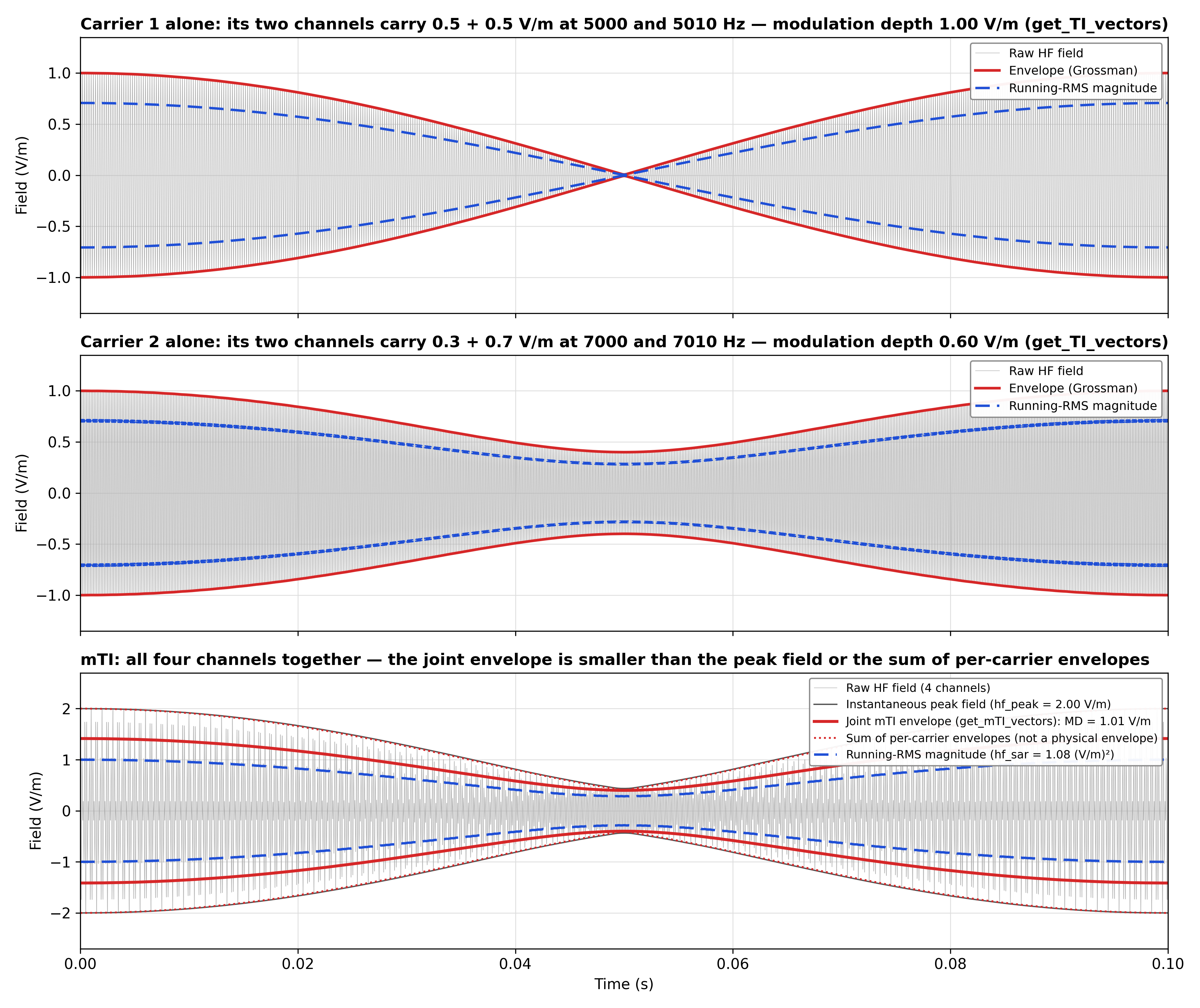 One point of an mTI field (4 channels, 2 beating pairs), with every channel field along one axis for clarity. Pair 1's channels carry 0.5 + 0.5 V/m, pair 2's 0.3 + 0.7 V/m. On its own, each pair's envelope amplitude is 1.00 and 0.60 V/m (top, middle). Together (bottom), the pairs' power envelopes add (not their amplitudes) and the joint envelope amplitude is 1.01 V/m (
envelope_max). The larger numbers are other quantities: the dotted sum of per-pair envelopes (2.00 V/m) is not a physical envelope, a TI-of-TI recombination would give 1.20 V/m, and hf_peak = 2.00 V/m is the instantaneous peak of the summed field. The dashed running RMS is the power view of the same field; its mean square is hf_power = 0.54 (V/m)², so hf_rms = 0.73 V/m (see Carrier fields).
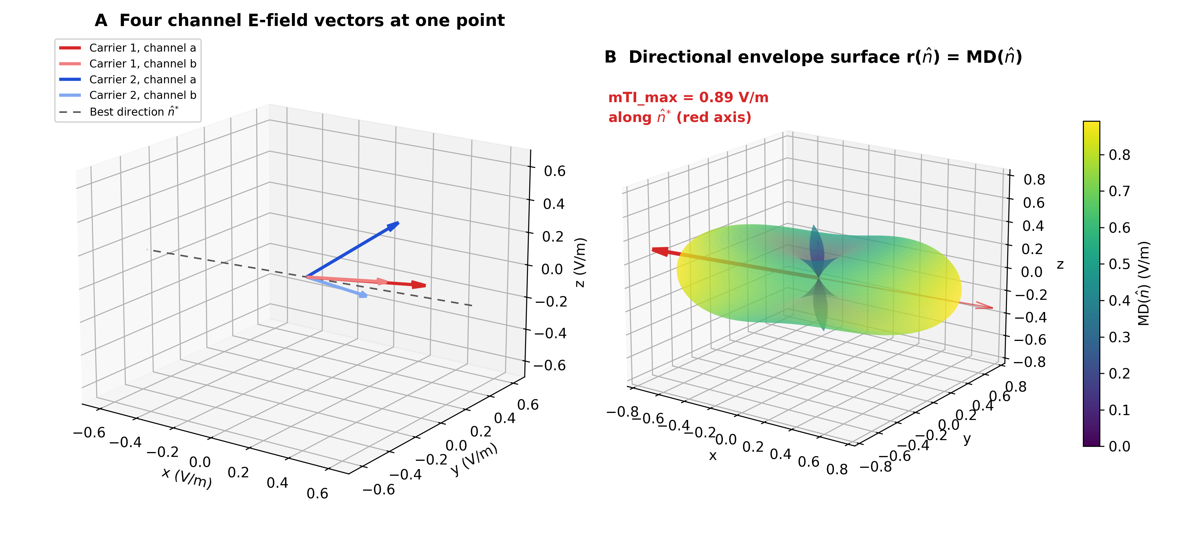 The same idea in vector space. (A) The four channel fields at one point. (B) The envelope amplitude along each direction, drawn as the radius \(r(\hat{\mathbf{n}}) = E_{\mathrm{AM}}(\hat{\mathbf{n}})\) (MD in the figure).
mTI_max is the radius of the farthest point, 0.89 V/m along \(\hat{\mathbf{n}}^{*}\) here, which envelope_max finds. TI_avg is the mean radius over all directions.
Two shortcuts give different and wrong numbers, and the toolbox offers neither: adding the per-pair envelopes (the pairs’ power envelopes add, not their amplitudes), and feeding per-pair envelopes back into the two-channel formula as if they were fields (TI-of-TI). How the toolbox tells a TI montage from an mTI montage is described on the Simulator page.
How each quantity is computed
Every quantity is exact except TI_max for \(K \ge 2\) (a numerical maximisation) and TI_avg for \(K \ge 2\) (a sphere quadrature):
Details: method and accuracy per quantity
| Quantity | tit.calc |
Two channels (\(K = 1\)) | More beating pairs (\(K \ge 2\)) |
|---|---|---|---|
TI_normal |
envelope |
exact (the expression above) | exact |
TI_max / mTI_max |
envelope_max |
exact closed form | the maximiser is an eigenvector of \(\cos\theta\,\mathbf{C}_+ - \sin\theta\,\mathbf{C}_-\) with \(\mathbf{C}_+ = \tfrac{1}{2}\mathbf{S}^\top\mathbf{S}\) and \(\mathbf{C}_- = \tfrac{1}{2}\mathbf{D}^\top\mathbf{D}\): a root-find along its three eigen-branches, then a local Newton polish. On \(10^4\) random elements per \(K = 2, 3, 4\) and \(4 \times 10^5\) real grey-matter elements, none came out more than \(10^{-6}\) (relative) below a dense reference search |
| tangential maximum | envelope_max(..., perpendicular_to=) |
exact (closed form on the in-plane fields) | exact (roots of a degree-6 polynomial) |
TI_avg |
envelope_mean |
exact closed form | 4096-direction sphere quadrature (2048 on a hemisphere, since \(E_{\mathrm{AM}}(\hat{\mathbf{n}}) = E_{\mathrm{AM}}(-\hat{\mathbf{n}})\)), about \(7 \times 10^{-4}\) relative error at worst |
hf_peak |
hf_peak |
exact, \(\max(\lVert \mathbf{E}_1 + \mathbf{E}_2 \rVert, \lVert \mathbf{E}_1 - \mathbf{E}_2 \rVert)\) | exact for any number of channels (every sign pattern up to eight channels, zonotope vertices above) |
hf_rms, hf_power_density |
hf_power |
exact | exact |
Carrier fields
hf_peak, hf_rms and hf_power_density describe the kHz carrier fields themselves rather than the envelope. They are computed by tit.calc.hf_peak and tit.calc.hf_power from all \(N\) channel fields \(\mathbf{E}_1, \dots, \mathbf{E}_N\). The two channels of a beating pair differ by \(\Delta f\), so no two channels share a frequency, and every channel field enters on its own. All E-fields, TI_max and hf_peak are zero-to-peak amplitudes for zero-to-peak channel currents; hf_rms is the RMS over time and hf_power its square, the time-averaged mean square.
hf_peak (\(HF_{peak}\), V/m) is the largest instantaneous magnitude the summed field can reach, zero-to-peak:
where each \(s_j\) is a crest (\(+1\)) or trough (\(-1\)) of channel \(j\). For two channels it is \(\max(\lVert \mathbf{E}_1 + \mathbf{E}_2 \rVert, \lVert \mathbf{E}_1 - \mathbf{E}_2 \rVert)\), Cassarà Part I, Eq. 3 (p. 11).
hf_rms (\(HF_{rms}\), V/m) is the RMS in-situ carrier field over time. Fields at different frequencies add in power, not amplitude (Cassarà Part I, p. 11; Part II, p. 8), so
hf_power_density (\(p_{HF}\), W/m³) is the absorbed (Joule) power density of the carriers, time-averaged, with the conductivity \(\boldsymbol{\sigma}\) the simulation solved with:
Details: why the sign maximum is the peak, conductivity, SAR, which fields are saved
The definitions follow Cassarà et al. 2025 (Bioelectromagnetics, Part I 46(2):e22542, doi:10.1002/bem.22542; Part II 46(1):e22536, doi:10.1002/bem.22536).
Each channel’s field oscillates between \(+\mathbf{E}_j\) and \(-\mathbf{E}_j\), and the magnitude of the sum is largest when every channel is at a crest or a trough, so the maximum over sign choices is the maximum over all phase combinations. The field reaches this peak when every phase combination occurs over time. With harmonically related carriers, such as channels at 2.000, 2.010, 4.000 and 4.010 kHz, some combinations never occur, and hf_peak is then an upper bound. The maximum is exact for any number of channels: it lies at a vertex of the zonotope spanned by the \(\pm\mathbf{E}_j\), and the candidate sign patterns are those around the directions \(\mathbf{E}_i \times \mathbf{E}_j\).
For isotropic (scalar) conductivity \(p_{HF}\) is \(\sigma \cdot \mathrm{hf\_power}\), with each tissue’s value including any overrides; for the anisotropic models (vn, dir, mc) each element’s full DTI conductivity tensor is used. It is not SAR: SAR is this divided by the tissue density, \(\mathrm{SAR} = p_{HF} / \rho\) (IEEE C95.1-2019, p. 35; Cassarà Part II, Eq. 1), and the toolbox does not apply \(\rho\). It is written on the volume mesh and its NIfTIs only, not projected to fsaverage: that projection interpolates the fields onto the cortical surface, not the conductivity.
A simulation saves TI_max, hf_peak and hf_rms by default; TI_avg and hf_power_density only when they are ticked (see Output Fields on the Simulator page). An analysis of a field the simulation did not save computes it first from the simulation’s channel meshes and saves it (Fields computed on demand), except hf_power_density, which needs the conductivity of the original solve and must be ticked before the run. The Analyzer treats each like any other field, in its own units.
Carrier-only controls (ΔF = 0)
A carrier-only control drives both channels of a two-channel montage at the same frequency (for example 15,000 / 15,000 Hz), phase-locked and in phase, so there is no beat and no envelope. The channels then add into one field \(\mathbf{E}_1 + \mathbf{E}_2\) oscillating at the carrier frequency. Following Cassarà Part II (p. 8: “coherent field superposition was used for identical frequencies”), the fields are summed as vectors first:
\[\mathrm{hf\_peak} = \lVert \mathbf{E}_1 + \mathbf{E}_2 \rVert, \qquad \mathrm{hf\_rms} = \tfrac{1}{\sqrt{2}} \lVert \mathbf{E}_1 + \mathbf{E}_2 \rVert, \qquad \mathrm{hf\_power\_density} = \tfrac{1}{2} (\mathbf{E}_1 + \mathbf{E}_2)^{\top} \boldsymbol{\sigma} \, (\mathbf{E}_1 + \mathbf{E}_2)\]TI_max, TI_avg and TI_normal are undefined without a beat and are not computed; a carrier-only run writes only hf_peak, hf_rms and/or hf_power_density. To set one up, in the app or from Python, see Carrier-only control on the Simulator page.
Details: how the carrier fields compare with a TI run
hf_peak keeps its TI value where the two fields are within 90° of each other and is smaller elsewhere. hf_power (\(\mathrm{hf\_rms}^2\)) gains the cross term \(\mathbf{E}_1 \cdot \mathbf{E}_2\), so it ranges from twice its TI value (equal, aligned fields) to zero (equal, opposed fields), and hf_rms from \(\sqrt{2}\) times its TI value to zero. For example, \(\lVert \mathbf{E}_1 \rVert = 1\) and \(\lVert \mathbf{E}_2 \rVert = 0.8\) V/m at 120° give hf_peak = 1.56 V/m in a TI run and 0.92 V/m in a carrier-only run. “In phase” follows the simulation’s sign convention: each channel’s first electrode is driven positive at the same instant.
Modulation and stimulation focality
roi_focality says how concentrated the modulation is in the target. A TI field is carried by kHz fields that are themselves spread over the head, and the premise of TI is that the modulation is more focal than they are. An analysis of a modulation field (TI_max, mTI_max, TI_avg or TI_normal) therefore also reports the focality of the stimulation intensity, from the same simulation, on the same elements:
where
- \(F_{\mathrm{TI}}\) is
roi_focality, \(F_{HF_{peak}}\)hf_peak_focality, \(F_{HF_{rms}}\)hf_rms_focalityand \(S_{\mathrm{TI}}\)ti_selectivity; - \(HF_{peak}\) and \(HF_{rms}\) are the saved fields
hf_peakandhf_rms; for mTI they run over every channel’s carrier; - \(\langle \cdot \rangle\) is the area-weighted (mesh) or volume-weighted (voxel) mean over exactly the target and reference elements of
roi_meanandgm_mean: the nodes or voxels where the analysed field is positive.
A TI_normal analysis divides TI_normal’s own focality by \(F_{HF_{peak}}\). Reading ti_selectivity: above 1, the modulation is more concentrated in the target than the carriers: the envelope adds focality that a kHz field alone does not have. At or below 1, a plain kHz field with the carriers’ spatial distribution reaches the target as selectively as the modulation does. The ratio compares spatial distributions only; it says nothing about how neurons respond to a kHz field compared with an envelope.
Ex-search reports the same two ratios for every candidate, as HFpeak_Focality and TI_Selectivity (Ex-search metrics).
Details: why RMS and not power, where the carrier fields come from, missing values
- Why \(HF_{rms}\) and not power. A field twice as strong in the target as in the reference has four times the power there. The ratio of mean powers would therefore be roughly the square of a field ratio, and not comparable with
roi_focality. \(HF_{rms}\) is a field strength (V/m), sohf_rms_focalityis a linear ratio likeroi_focalityandhf_peak_focality. - Where the carrier fields come from. The Analyzer reads
hf_peakandhf_rmsfrom the same outputs as the analysed field: in mesh space the central surface, which carries every field of the TI or mTI mesh, and in voxel space the NIfTI of the same tissue (grey_<sim>_TI_subject_hf_peak.nii.gzbesidegrey_<sim>_TI_subject_TI_max.nii.gz). They go through the same interpolation as the modulation field. A simulation saves both by default; one that did not has them computed and saved by the analysis first (on_demand_notesays so), into its field mesh before the central surface is regenerated, so they still share the modulation field’s interpolation. - When one has no usable values. A carrier field with NaN or infinite values on the analysed elements, a carrier whose reference mean is 0, or a carrier NIfTI on another grid (shape or affine) leaves its statistics empty, with the reason in
carrier_note, and the Analyzer logs one warning. Nothing is approximated, and the modulation statistics are never affected. An analysis of a carrier field (hf_peak,hf_rms,hf_power_density) has no carrier statistics, andcarrier_notesays so. When the simulation can neither provide nor compute a carrier (its channel meshes are gone, or only its NIfTIs were kept), those statistics are empty andcarrier_notesays what is missing; the modulation statistics are still reported.