Analyzer Module

The Analyzer is the last step of the pipeline: after a montage has been optimized (flex-search, ex-search) and simulated, it turns the finished simulation into numbers — descriptive statistics of the field inside a region of interest and across the whole brain, in mesh or voxel space. One Analyzer class handles both spaces, and run_group_analysis() extends the same analysis across subjects and montages.

This page is also where the toolbox’s field quantities are defined once for everyone: the optimizer and simulator pages link here for what TI_max, TI_normal, TI_avg, hf_peak and hf_sar mean and how the envelope math works.

Overview

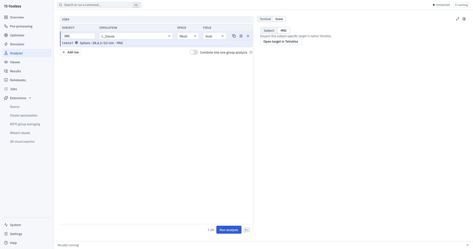The Analyzer (⌘4). One row is one analysis, and each row owns its own target.

---

Quantities of Interest

Two words carry all of the structure on this page. A channel is one pair of electrodes driven by one current source at one kHz frequency. Two channels at slightly offset frequencies share a carrier and produce one beat: standard TI is 4 electrodes forming 2 channels on one carrier (e.g. 2.000 and 2.010 kHz around a 2 kHz carrier), and mTI is 8 electrodes forming 4 channels on two carriers (e.g. 2 kHz and 4 kHz — each pair of channels shares one).

Neither channel’s kHz field modulates neurons on its own; the quantity the TI community cares about is the amplitude of the low-frequency beat that the two channels sharing a carrier produce where their fields overlap. Everything the analyzer reports is a spatial statistic of that one quantity, so it helps to see it once in the time domain and once in the spatial domain.

Time domain: what a single value of TI_max is

The kHz fields of two channels sharing a carrier, each too fast to modulate neurons on its own, sum where they overlap into a field whose amplitude beats at the difference frequency. The peak-to-trough swing of that envelope is the modulation depth -- the single number TI_max stores at every mesh node or voxel.

• TI_max (V/m) – the modulation depth of the beat envelope, maximised over direction at every mesh node or voxel. It is the default field of every simulation and of every analysis, and what “TImax” / “TInorm” mean in papers and in this toolbox’s optimizers. For one carrier (two channels) it is the closed form \(2\min(\lVert \mathbf{E}_1 \rVert, \lVert \mathbf{E}_2 \rVert)\) when the fields are near-aligned, and smaller otherwise (Grossman et al. 2017; exact form under Envelope Math and Critical Values below).
• TI_normal (V/m, mesh only) – the same envelope measured along the local cortical surface normal, i.e. the component that runs along the apical dendrites of pyramidal cells. It is always \(\le\) TI_max, can be much smaller where the field is tangential to the cortex (see below), and is written for both TI and mTI runs (for mTI via get_TI_dir, the same envelope evaluated along the surface normal).
• TI_avg, hf_peak, hf_sar – optional extra fields (direction-averaged envelope; carrier-exposure safety metrics). They are defined below (Envelope Math and Safety Metrics); the analyzer treats them as any other field, each in its own units.

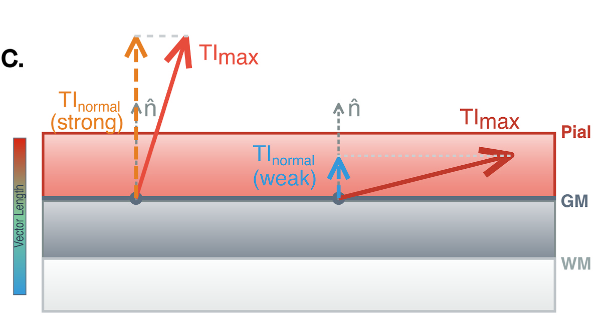At each surface node, TI_normal is the component of the TI_max envelope along the local surface normal \(\hat{n}\): where the field runs along \(\hat{n}\) (left) the two are nearly equal, and where it runs tangential to the cortex (right) TI_normal collapses even though TI_max is unchanged. Figure 4C from Haber et al. 2026.

Multipolar (mTI): more carriers, same quantity

With four channels on two carriers (8 electrodes) — or more — mTI_max is still the same beat-envelope modulation depth: each carrier’s two channels beat exactly as in standard TI, and the carriers, being mutually incoherent, add powers, not amplitudes:

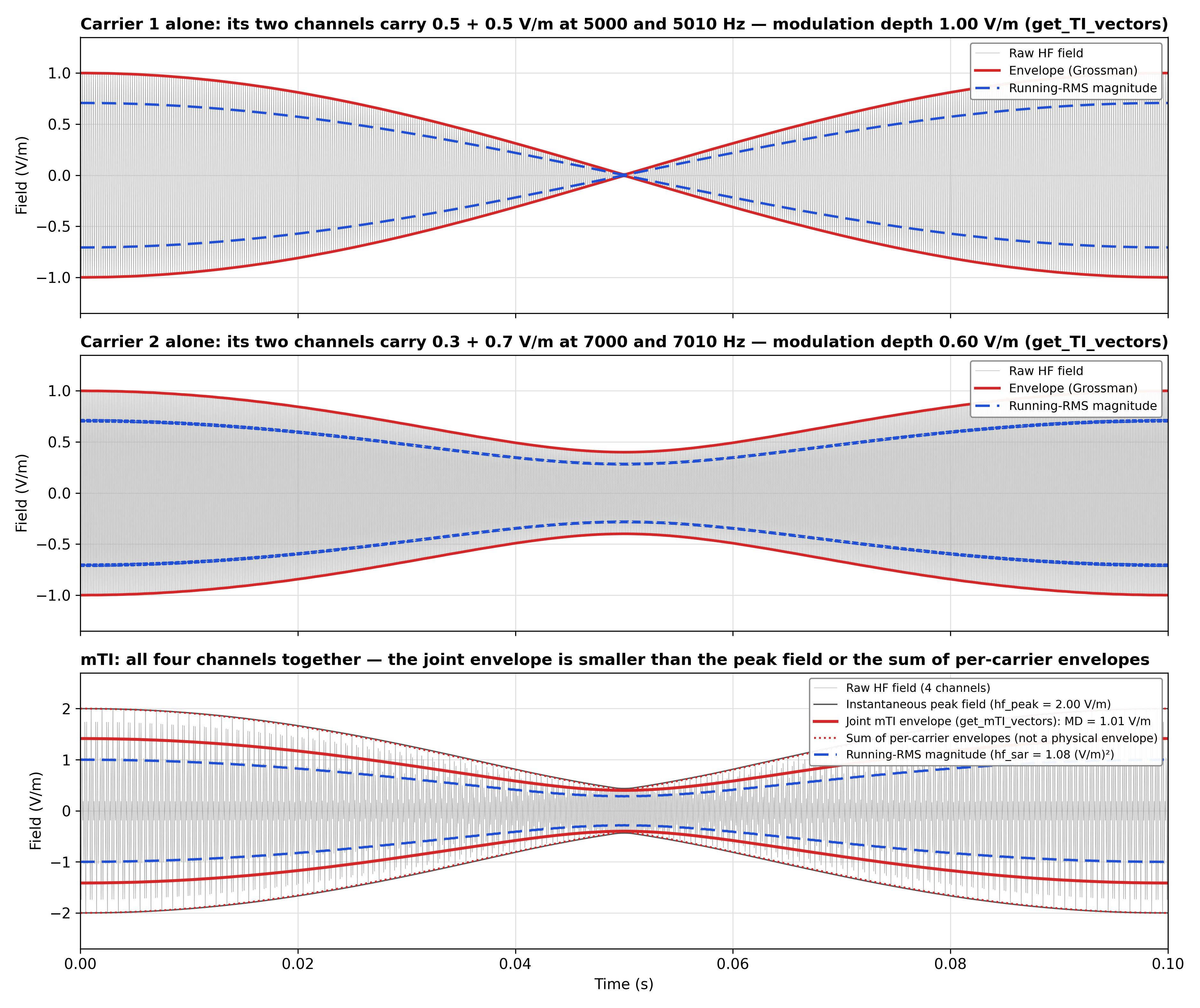Time domain of an mTI field (4 channels, 2 carriers) at one point, all projections colinear for clarity: carrier 1's two channels carry 0.5 + 0.5 V/m, carrier 2's an unequal 0.3 + 0.7 V/m (so its beat never reaches zero). Alone, each carrier's modulation depth is 1.00 and 0.60 V/m (top, middle; get_TI_vectors). With all four channels together (bottom), the two carriers are mutually incoherent, so the joint envelope adds their powers, not their amplitudes: get_TI_vectors gives MD = 1.01 V/m. Every larger quantity in the panel is a different thing: the dotted sum of per-carrier envelopes (peaking at 2.00 V/m) is not a physical envelope; a recursive TI-of-TI recombination would report an unphysical 1.20 V/m; and the worst-case instantaneous peak of the summed channel fields hf_peak = 2.00 V/m is a safety quantity, not a modulation depth. The dashed running-RMS magnitude is the power view of the same field (its square relates to hf_sar = 1.08 (V/m)²; see Safety Metrics). All values verified against tit.calc/tit.fields for this exact scenario.

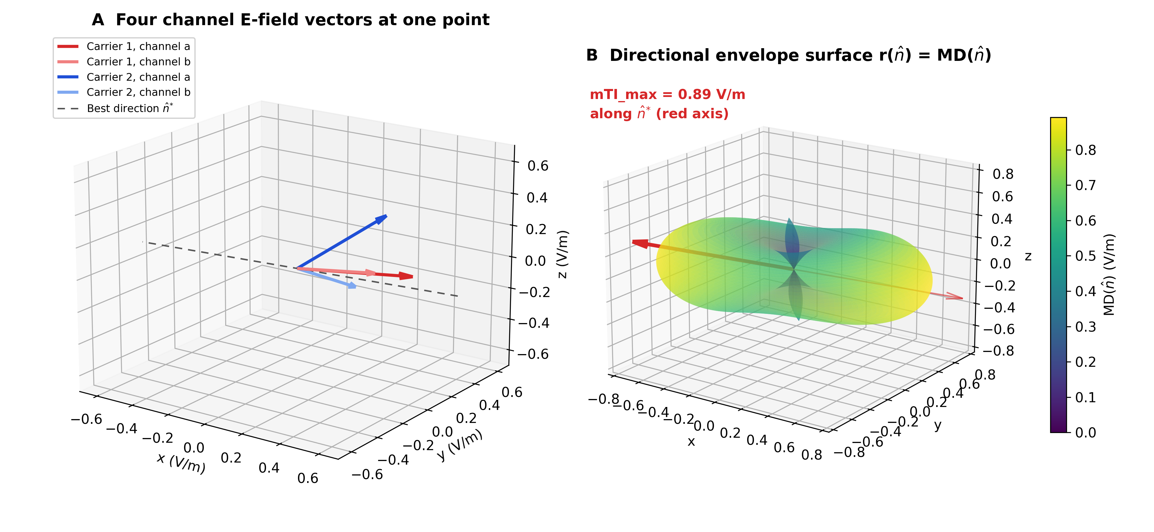The same idea in vector space. At each mesh element the four channels' E-fields are vectors (A), and the modulation depth depends on the direction \(\hat{n}\) it is measured along: sweeping \(\hat{n}\) over the sphere and plotting \(r(\hat{n}) = \mathrm{MD}(\hat{n})\) from the \((P, Q)\) formulas gives the directional envelope surface (B). mTI_max is the radius of this surface's farthest point -- exactly what get_TI_vectors finds with its 192-direction Fibonacci sweep plus local refinement (0.89 V/m along \(\hat{n}^{*}\) here, verified against the toolbox for these vectors). TI_avg is the average radius of the same surface over all sampled directions.

The two subsections below give the formulas behind these figures – the \((P, Q)\) sufficient statistics, the exact one-carrier closed form, and the safety metrics. How montages are detected as TI vs. mTI is a simulation mechanic covered on the Simulator page.

Envelope Math and Critical Values

The envelope for any number of carriers \(K\) reduces to two sufficient statistics of the channel fields’ projections onto a candidate direction \(\mathbf{n}\). For carrier \(k\), the signed projections of its two channels’ fields are

\[a_k = \mathbf{E}_{ka} \cdot \mathbf{n}, \qquad b_k = \mathbf{E}_{kb} \cdot \mathbf{n}\]

from which the carrier power \(P\) and the coherent phasor sum \(Q\) follow:

\[P = \frac{1}{2} \sum_k \left( a_k^2 + b_k^2 \right), \qquad Q = \left\lvert \sum_k a_k b_k \, e^{i \psi_k} \right\rvert\]

and the modulation depth is

\[\mathrm{MD} = \sqrt{2} \left( \sqrt{P + Q} - \sqrt{P - Q} \right)\]

\(\psi_k\) is a per-carrier envelope phase offset (radians), None by default (all carriers phase-aligned, \(\psi_k = 0\), the standard case). \(P - Q\) and \(P + Q\) are clamped to \(\ge 0\) before the square roots to absorb floating-point round-off. This is implemented in tit/calc.py, whose public API is exactly three functions:

Function	Purpose
get_TI_vectors(fields, psi=None)	Modulation-amplitude vectors for \(K \ge 1\) carriers (\(K = 1\) exact closed form, \(K \ge 2\) direction search)
get_TI_avg(fields, psi=None)	Direction-averaged modulation depth
get_TI_dir(fields, directions, psi=None)	Envelope along a fixed per-element direction; backs TI_normal for mTI

get_TI_vectors is the one envelope function; standard TI simulation, mTI simulation and mex-search all call it. It takes fields = [E_1a, E_1b, ..., E_Ka, E_Kb] – one array of shape (N, 3) per channel, ordered so that consecutive fields are the two channels sharing a carrier – and returns (N, 3) modulation-amplitude vectors whose norm is \(\mathrm{MD}\).

• \(K = 1\) (one carrier: standard TI) is solved by an exact closed form (Hirata et al. 2024, Computers in Biology and Medicine 178, 108697; sign-agnostic):

  \[\mathrm{MD} = \begin{cases} 2 \min\!\left( \lVert \mathbf{E}_1 \rVert, \lVert \mathbf{E}_2 \rVert \right) & \text{if } \min\!\left( \lVert \mathbf{E}_1 \rVert, \lVert \mathbf{E}_2 \rVert \right) \le \sqrt{\lvert \mathbf{E}_1 \cdot \mathbf{E}_2 \rvert} \\[8pt] \dfrac{2 \lVert \mathbf{E}_1 \times \mathbf{E}_2 \rVert} {\min\!\left( \lVert \mathbf{E}_1 - \mathbf{E}_2 \rVert, \lVert \mathbf{E}_1 + \mathbf{E}_2 \rVert \right)} & \text{otherwise} \end{cases}\]

  In the first case the envelope lies along the smaller field’s own (sign-corrected) direction; in the second it is evaluated at the component of the smaller field perpendicular to whichever of \(\mathbf{E}_1 - \mathbf{E}_2\) / \(\mathbf{E}_1 + \mathbf{E}_2\) has the smaller norm. No direction search is needed at \(K = 1\).

• \(K \ge 2\) (multiple carriers: mTI) has no closed form and is solved by a direction search: a coarse 192-point Fibonacci-sphere sweep (num_directions=192), followed by 3 rounds of local patch refinement around up to 6 angularly-diverse coarse-sweep seeds (_REFINE_N_ROUNDS=3, _REFINE_N_SEEDS=6, minimum seed separation _REFINE_MIN_SEED_ANGLE_DEG=25.0, 16 points per patch, initial half-angle \(2.0/\sqrt{192}\) radians shrinking by 0.4 each round). Elements are processed in chunks of 16384 to bound memory. get_TI_avg reuses the same coarse sweep but averages the envelope over all 192 sampled directions instead of taking the per-element argmax, and skips refinement (refinement only sharpens a single best direction, which an average does not need) – it is element-wise \(\le \mathrm{TI}_{\max}\).

The same modulation depth \(\mathrm{MD}(\mathbf{n}) = \sqrt{2}\left(\sqrt{P + Q} - \sqrt{P - Q}\right)\) answers three different questions, and the three functions differ only in what they do with the direction \(\mathbf{n}\):

• get_TI_vectors — maximise over \(\mathbf{n}\): the strongest modulation any neuron at that point could see, whatever its orientation. This is TI_max / mTI_max, and what the optimizers score.
• get_TI_dir — evaluate at a given \(\mathbf{n}\): the modulation seen along one specific orientation. With \(\mathbf{n}\) set to the cortical surface normal this is TI_normal, the component along pyramidal-cell dendrites.
• get_TI_avg — average over all \(\mathbf{n}\): what a randomly-oriented neuron sees on average. This is TI_avg, and it is always \(\le\) TI_max.

Two tempting shortcuts are not valid and are deliberately not offered: summing the per-carrier envelopes (carriers are mutually incoherent, so their powers add, not their amplitudes — the dotted trace in the time-domain figure above overshoots the physical envelope) and recombining per-carrier envelopes recursively as TI-of-TI (an envelope is not a field; feeding one back into the one-carrier formula is physically invalid).

Safety Metrics

Two carrier-exposure safety metrics (tit/fields.py, Cassarà et al. 2025, Bioelectromagnetics 46(2), doi:10.1002/bem.22542) are computed directly from the N per-channel E-fields, independent of the modulation-depth envelope:

hf_peak (Eq. 3) is the worst-case instantaneous peak of the summed kHz field: the channels run at mutually incommensurate frequencies, so every relative phase combination occurs over time, and the true worst case is the max over sign choices,

\[\mathrm{hf\_peak} = \max_{\mathbf{s}} \left\lVert \sum_i s_i \mathbf{E}_i \right\rVert, \qquad s_i \in \{ +1, -1 \}\]

At \(N = 2\) this is exactly \(\max\!\left( \lVert \mathbf{E}_1 + \mathbf{E}_2 \rVert, \; \lVert \mathbf{E}_1 - \mathbf{E}_2 \rVert \right)\). Up to EXACT_SIGN_ENUM_MAX_FIELDS = 8 fields, this is solved by exact sign enumeration (\(2^{N-1}\) combinations – 128 at \(N = 8\)). Above 8 fields the combinatorics blow up (measured ~44.6s for \(N = 12\)’s 2048 combinations at 200k elements vs. ~2.0s at \(N = 8\)), so a 4000-direction Fibonacci-sphere sweep picks the best-sampled support direction and evaluates the exact, realizable vector sum for the sign pattern it implies. This sweep fallback is still a lower bound on the true max over all \(2^{N-1}\) sign combinations – since only the sampled directions’ implied patterns are tried – and is therefore slightly non-conservative.

hf_sar is the incoherent sum of the channel-field powers, in \((\mathrm{V/m})^2\) – power adds rather than amplitude:

\[\mathrm{hf\_sar} = \sum_i \lVert \mathbf{E}_i \rVert^2\]

This is a field-domain heating proxy, not calibrated SAR: the actual calibration is \(\tfrac{\sigma}{2\rho} \cdot \mathrm{hf\_sar}\), requiring the per-tissue conductivity \(\sigma\) and density \(\rho\) that the toolbox does not apply.

Under the shipped positional wiring, each field is one carrier, so both metrics include every channel field. Shared-frequency fields would require coherent vector summation first. Both metrics are opt-in: neither is in SimulationConfig.output_fields’s default (["TI_max"]), so a run must explicitly request hf_peak/hf_sar to get them written.

Spatial domain: how the analyzer summarises a field

Once TI_max exists at every node or voxel, an analysis reduces it to a handful of spatial statistics – intensity inside the target, intensity everywhere else, and how concentrated the hot spot is:

Quantity	AnalysisResult field	What it tells you
Intensity in the ROI	roi_mean (also roi_max, roi_min)	Area/volume-weighted mean TI_max inside the target. The number to compare against dose thresholds and between montages.
Intensity outside the ROI	gm_mean (also gm_max)	Mean over the entire grey matter. This is the analyzer’s fixed non-ROI; the optimizers additionally accept a user-defined avoidance region.
Focality	roi_focality	roi_mean / gm_mean. 1 means the target is no hotter than the average cortex; higher is more selective. Same definition as ex-search’s Focality.
Normal component	normal_mean, normal_max, normal_focality	The three statistics above recomputed on TI_normal (mesh only).
Hot-spot level	percentile_95, percentile_99, percentile_99_9	Field value below which 95 / 99 / 99.9 % of the grey-matter area lies. percentile_99_9 is a robust “peak” that ignores single outlier elements.
Hot-spot size	focality_50_area … focality_95_area	Grey-matter area (\(\mathrm{cm}^2\); volume for voxel analysis) at or above 50 / 75 / 90 / 95 % of percentile_99_9. A small focality_50_area means a compact hot spot; a large one means the field is spread out, regardless of where the ROI is.

Two things trip people up: the percentile and area metrics are whole-cortex descriptors and do not depend on the ROI at all, and every statistic is computed on whichever field you selected, in that field’s units – selecting hf_sar gives you means of a power-like quantity in \((\mathrm{V/m})^2\), not a field strength.

---

Defining the ROI

An analysis needs a target region. The same ROI picker used by the optimizers offers spherical, cortical (atlas), and subcortical definitions:

Spherical ROI Analysis

• Analyze field data within spherical regions of interest
• Customizable center coordinates and radius
• Multiple spheres: type x,y,z,r and press Enter / Add Sphere — each sphere becomes a removable chip. By default every sphere runs as its own separate analysis — N spheres produce N independent result sets
• Combine spheres into one ROI: tick this and the spheres are unioned into a single ROI, giving one analysis and one result set for all of them (overlapping spheres are not double-counted). The output folder is named spheres<N>_..., and long unions are shortened to the first sphere plus a hash
• Group analysis runs one ROI across all subjects: several spheres are accepted only when they are combined, otherwise extra spheres are rejected with a warning
• Support for subject-space and MNI coordinates (automatic transformation)

Cortical Analysis (Region Union)

• Analyze one or more atlas regions as a single combined ROI — passing more than one region name unions their masks into one target, and the result’s region name is the selected names joined with +
• Combine regions into one ROI (GUI, on by default): untick it to run one separate analysis per selected region instead of a union. Group analysis requires the combined form when more than one region is selected
• In mesh space, a bare region name (e.g. cuneus) expands to both hemispheres (lh.cuneus + rh.cuneus)
• Mesh atlases: DK40, a2009s, HCP_MMP1. Voxel atlases: aparc.DKTatlas+aseg.deep.mgz (the cortical DKT parcellation FastSurfer’s --seg_only produces when optional FastSurfer segmentation is run), plus the subject’s own segmentation/labeling.nii.gz (charm; also gives whole-thalamus/-hippocampus/-amygdala). Five more voxel atlases only ever exist for a subject with derivatives/freesurfer/ output from a FreeSurfer recon-all run — aparc.DKTatlas+aseg.mgz, aparc.a2009s+aseg.mgz, lh.hippoAmygLabels-T1.v22.mgz, rh.hippoAmygLabels-T1.v22.mgz, ThalamicNuclei.v13.T1.mgz — and are absent for a FastSurfer-only subject, with optional FreeSurfer subregion processing available separately; see Pre-processing for what changed and why
• The four bundled MNI atlases (used elsewhere for subcortical ROI targeting) are not offered by the analyzer

Tissue Selection

• A Tissue selector (Gray Matter / White Matter / GM + WM) applies to voxel space only — it is disabled and forced to GM whenever Space is set to Mesh
• In voxel mode, the tissue choice selects which field file is loaded by filename prefix (grey_ for GM, white_ for WM, no prefix for GM + WM) and builds the corresponding tissue mask

---

Mesh-Based Analysis

When space="mesh", the Analyzer works with SimNIBS mesh files and provides high-resolution analysis of field data on brain surfaces.

Features

• Surface Mesh Generation: Automatic creation of gray matter surface meshes via msh2cortex (cached per instance)
• Atlas Integration: Support for SimNIBS native atlases (DK40, a2009s, HCP_MMP1)
• 3D Visualization: Generation of mesh files for 3D viewing

Cortical ROI Analysis

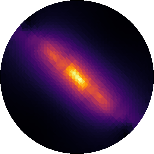
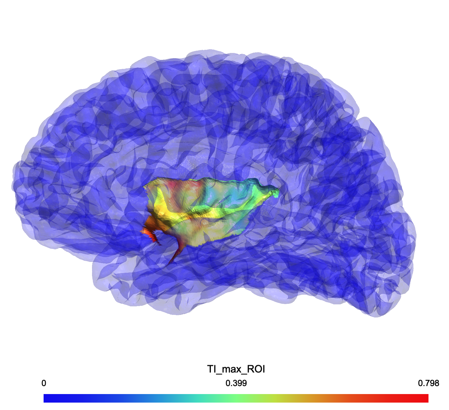TInorm field distribution in ROI (Left Insula)

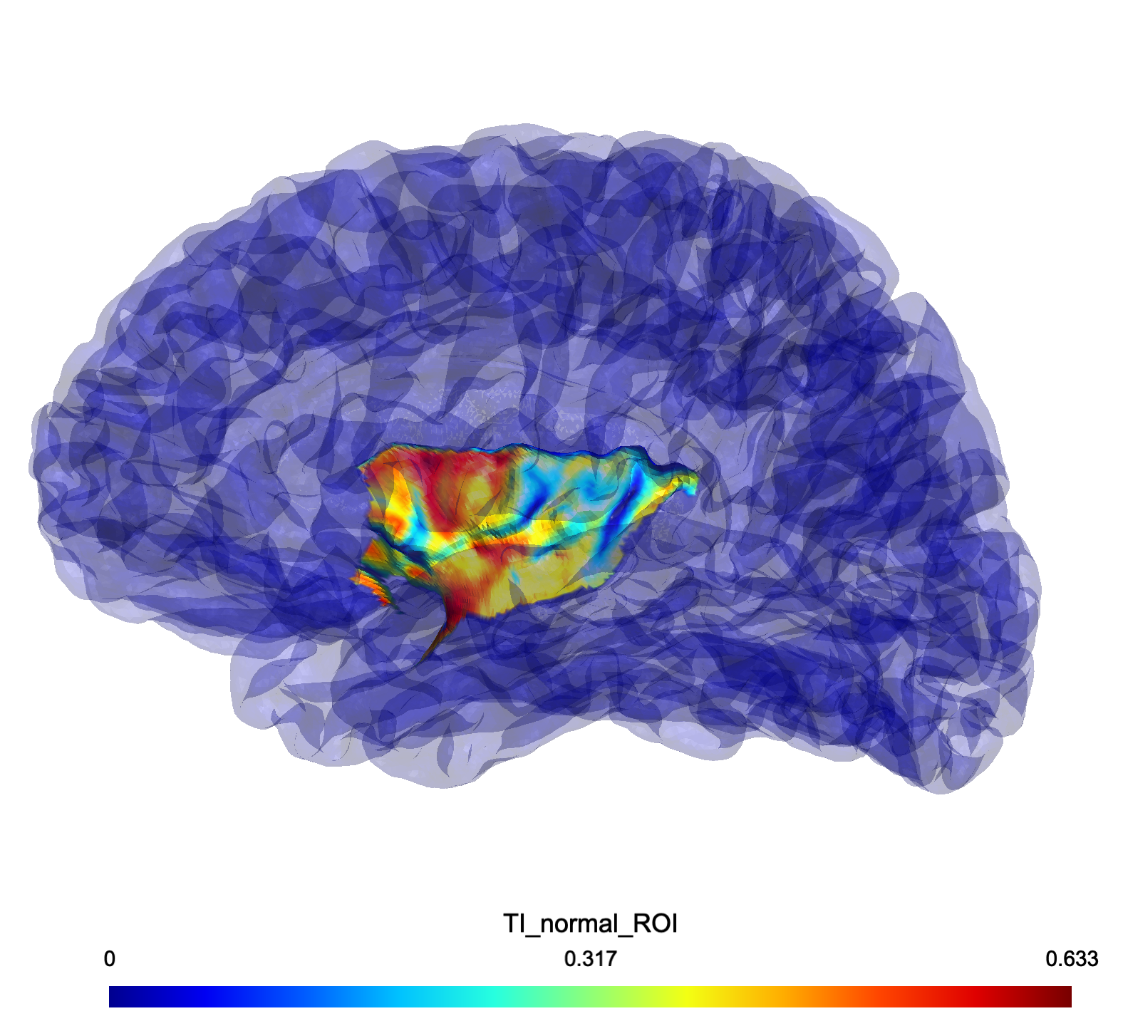TInormal field distribution in ROI (Left Insula)

Spherical ROI Analysis

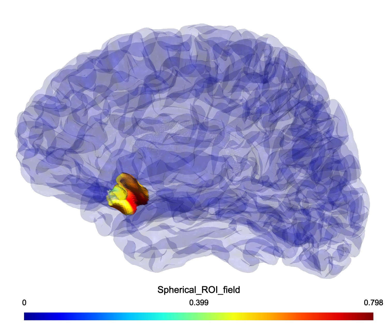Spherical ROI analysis showing TI_max field distribution within a 10mm radius sphere at coordinates (-31.3, 24.0, -37.0)

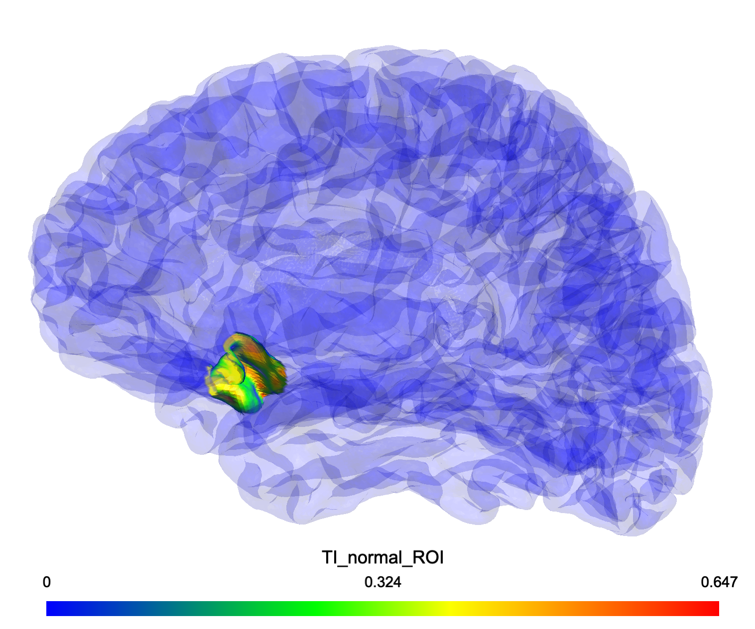Spherical ROI analysis showing TI_normal field distribution for the same target region, demonstrating directional field components

---

Voxel-Based Analysis

When space="voxel", the Analyzer handles NIfTI format files and integrates with FreeSurfer atlases for detailed volumetric analysis.

Features

• NIfTI Support: Direct analysis of .nii, .nii.gz, .mgz files
• FreeSurfer Integration: Automatic atlas region extraction and resampling
• Visualization Overlays: Generation of ROI-specific NIfTI overlays

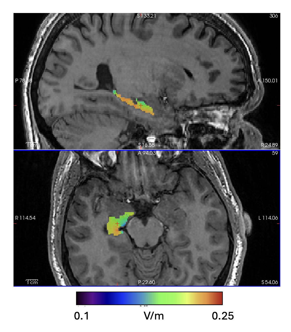Right Hippocampus ROI analysis showing TI_max field distribution given a 1mA:1mA stimualtion

---

What an analysis writes

One folder per analysis, under Analyses/<Mesh|Voxel>/<name>/, holding the data, the field-distribution histogram and exactly one scene:

File	What it is
results.csv	every statistic in the AnalysisResult, one row each
analysis.json	the target and settings the run used
roi_overlay.msh + .msh.opt (mesh)	the central surface with <field>_ROI node data: the field at the ROI’s nodes, exactly 0 everywhere else (and TI_normal_ROI when the run had a normal field)
roi_overlay.nii.gz (voxel)	the field, zero outside the ROI, on the field’s own grid
histogram.png	the whole-grey-matter field distribution — area-weighted (mesh) or volume-weighted (voxel) — with every bar coloured by the fraction of it inside the ROI (blue → red, colour bar), the ROI mean and the focality cutoffs (50/75/90/95 % of the GM 99.9th percentile) marked, and a whole-head / ROI stats box
scene.tetravox.json	a Tetravox scene of the overlay: in voxel space the field over your T1.nii.gz; in mesh space the whole cortex translucent with the ROI’s field coloured on top, cursor on the ROI, colour bar on
scene.png	a picture of that scene, when Tetravox is installed on the machine running the app

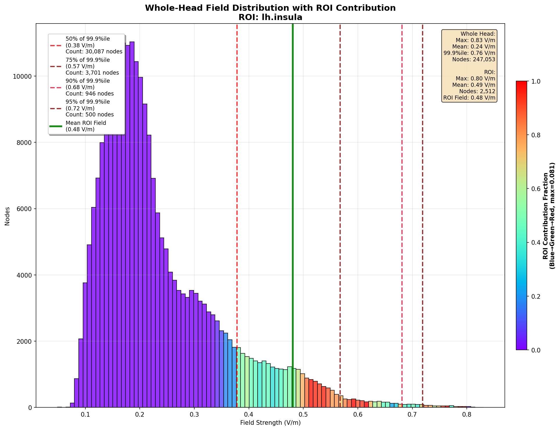Example field-distribution histogram, including target statistics and whole-grey-matter focality thresholds.

The scene is a few kilobytes and points at the overlay and the T1 — nothing is copied. Open it from the job’s Results row (Open in Tetravox) or by double-clicking the file.

AnalysisResult Fields

Every analysis call returns an AnalysisResult dataclass. Its statistics are exactly the quantities in the Quantities of Interest table, under the same names (roi_mean, gm_mean, roi_focality, normal_*, percentile_*, focality_*_area). The remaining fields identify and size the analysis:

• field_name, region_name, space (“mesh”/”voxel”), analysis_type (“spherical”/”cortical”)
• n_elements: mesh nodes or voxels in the ROI
• total_area_or_volume: ROI area (mesh, \(\mathrm{mm}^2\)) or volume (voxel, \(\mathrm{mm}^3\))
• The normal_* fields are None in voxel space, and for runs that predate TI_normal support for their mode – see mTI Analyses

Voxel-space focality_*_area values written by v2.3.0-v2.5.0 are 10x too large – they were computed in “cm^2” from a volume. v3.0.0 reports them in \(\mathrm{cm}^3\); see release notes (SCI-03) for whether to re-run or rescale.

---

mTI Analyses

The analyzer handles multipolar (mTI) simulations with the same Analyzer class, the same analyze_sphere / analyze_cortex / analyze_spheres calls, and the same ROI types — there is no mTI mode to select. The only signal it uses is whether {simulation}/mTI/mesh/ exists on disk.

What it reads

Space	mTI source	Standard TI source
Mesh	mTI/mesh/surfaces/{sim}_mTI_central.msh (field values)	TI/mesh/surfaces/{sim}_TI_central.msh
Voxel	mTI/niftis/ (grey_ / white_ prefix per tissue)	TI/niftis/

An mTI run also writes the intermediate per-carrier envelopes (TI_AB, TI_CD, …) into TI/mesh/. Those are not what the analyzer reads and are not the mTI result — each is only the two-channel envelope of one carrier on its own.

What mTI_max means for the statistics

mTI_max is the joint modulation depth over all \(K\) carriers at once, maximised over direction – the same “beat envelope” quantity as TI_max, just with more carriers in the sum. The math and the safety metrics are documented under Quantities of Interest above. What matters for analysis is:

• TI_max and mTI_max are aliases. Whichever spelling is requested, the analyzer resolves it to the on-disk name the detected simulation type actually wrote, so the Field selector lists it once.
• TI_avg, hf_peak and hf_sar can be selected when the run wrote them and go through the identical ROI machinery, each in its own units (see Quantities of Interest).

TI_normal

TI_normal is computed for mTI: the simulator evaluates the \(K\)-carrier envelope along the cortical surface normal (get_TI_dir) and writes {simulation}_mTI_normal.msh under mTI/mesh/. The analyzer resolves that mesh when TI_normal is requested for an mTI run, and the normal_* statistics (normal_mean, normal_max, normal_focality) are populated the same way as for standard TI. For mTI simulations run before this support existed, the normal mesh is absent — requesting TI_normal raises FileNotFoundError, and the normal_* statistics are None; re-run the simulation to get them.

---

Group Analysis

The run_group_analysis() function enables batch processing and comparative analysis across multiple subjects and montages, returning a GroupResult object.

Flexible Group Combinations

Group analysis supports arbitrary combinations of subjects and montages:

• Same subject x Multiple different montages: Compare different stimulation configurations within the same individual
• Multiple subjects x Same montage: Assess inter-subject variability for a specific stimulation protocol
• Multiple subjects x Different montages: Full factorial design comparing both subject variability and montage effects

MNI coordinates are transformed to each subject’s native space automatically, and every run produces cross-subject comparisons, rankings, and visualizations with consolidated logging.

---

Looking at a mesh analysis

When an analysis finishes, open it from Results — the mesh and the NIfTI outputs both open in the Viewer, in the application window. Both mesh-based analysis types are supported:

• Spherical ROI analyses with generated mesh overlays
• Cortical region analyses with atlas-based parcellations

What’s new in v3. 2.x launched Gmsh as a separate X11 program to inspect a mesh result, and Freeview for a NIfTI one. Both are gone — the container ships neither, and there is no X11 anywhere. Viewing is Tetravox, in the app.

Two more changes to the Analyzer itself: each row of the jobs table owns its own target, so one submission can analyse different ROIs across subjects; and a group run is refused unless every row agrees on simulation, space, field and target, with the disagreement named — it is never silently resolved to the first row.

Full list: the v3.0.0 release notes.

There is no separate “whole head” analysis type — the Analyzer supports only analysis_type spherical and cortical; the whole-GM statistics (gm_mean, gm_max, the percentiles and focality areas) and the ROI-vs-grey-matter histogram.png come with every analysis (mesh or voxel).

Custom NIfTI mask targets

Choose NIfTI mask in a job’s Target editor and import a .nii or .nii.gz file. All positive voxels belong to the target. Declare Subject or MNI explicitly: subject masks retain their coordinates, while MNI masks use the subject’s nonlinear m2m registration and nearest-neighbor sampling. Group analysis requires an MNI mask, registered separately for each subject.

Mesh analysis samples the mask at gray-matter surface nodes and reports surface-area statistics. Voxel analysis samples it onto the subject field grid and intersects it with the tissue selected in the job settings, retaining volume statistics. An empty overlap fails with a clear error. The script equivalent is analyzer.analyze_mask(mask_path, coordinate_space="mni"); job JSON uses analysis_type="mask", mask_path, and coordinate_space.

Target preview

The Scene pane follows the active job. Cortical atlas regions remain clickable. Masks, subcortical regions and spheres show a read-only target extent on subject anatomy; edit the target in its form. This previews the geometry, before the analysis applies its tissue and mesh settings. Incomplete targets or unavailable registration show an explanatory message.