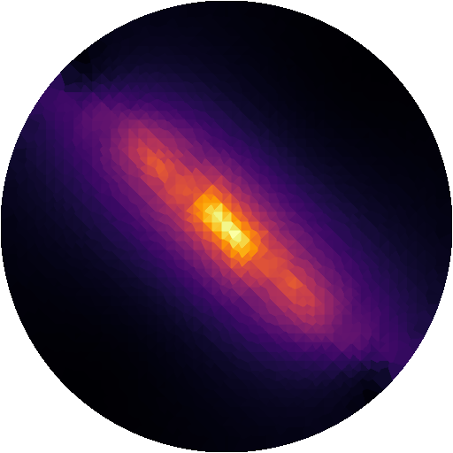
Flex Search Electrode Optimization

References:

• Original Paper: Weise K, Madsen KH, Worbs T, Knösche TR, Korshøj A, Thielscher A. A Leadfield-Free Optimization Framework for Transcranially Applied Electric Currents

• SimNIBS Implementation: Leadfield-free TES Optimization Tutorial

• Haber, I., Jackson, A., Thielscher, A., Hai, A., & Tononi, G. TI-Toolbox: An Open-Source Software for Temporal Interference Stimulation Research. Brain Stimulation

Job settings

Current ratio and Ratio total current sit together in the Electrode settings. Solver options are directly exposed, and After the search shows its options without opening a disclosure.

Run names

Leave the run name blank to use the current date and time. The application resolves one folder for both the preview and submission; simultaneous rows receive distinct suffixes. After submission, the next automatic run gets a fresh name. Enter a name to use that folder under the subject’s flex-search directory instead. Existing-output checks still apply.

Overview

Flex Search uses differential evolution optimization to determine the best electrode positions for TI stimulation. The public API is run_flex_search(config: FlexConfig) -> FlexResult, with all configuration expressed through type-safe dataclasses and enums.

Core capabilities:

• Desktop goals: Mean TImax (mean, average in the ROI), Max TImax (max, 99.9th percentile in the ROI), Threshold-free focality (focality_tf, weighted mean ROI / mean non-ROI), and Threshold-based focality (focality, ROC scoring).
• Post-processing Methods (FieldPostproc enum): max_TI, dir_TI_normal, or dir_TI_tangential
• ROI Definition: FlexConfig.SphericalROI, FlexConfig.AtlasROI, or FlexConfig.SubcorticalROI dataclasses – see Defining the ROI below
• Anisotropy Support: Four conductivity models (scalar, vn, dir, mc) with configurable max ratio and conductivity
• Multi-start Optimization: Run multiple optimization iterations and automatically select the best result
• Structured Output: Every run writes a flex_meta.json manifest for downstream consumption

In the application

Flex-search is the Flex method on the Optimizer page (⌘2).

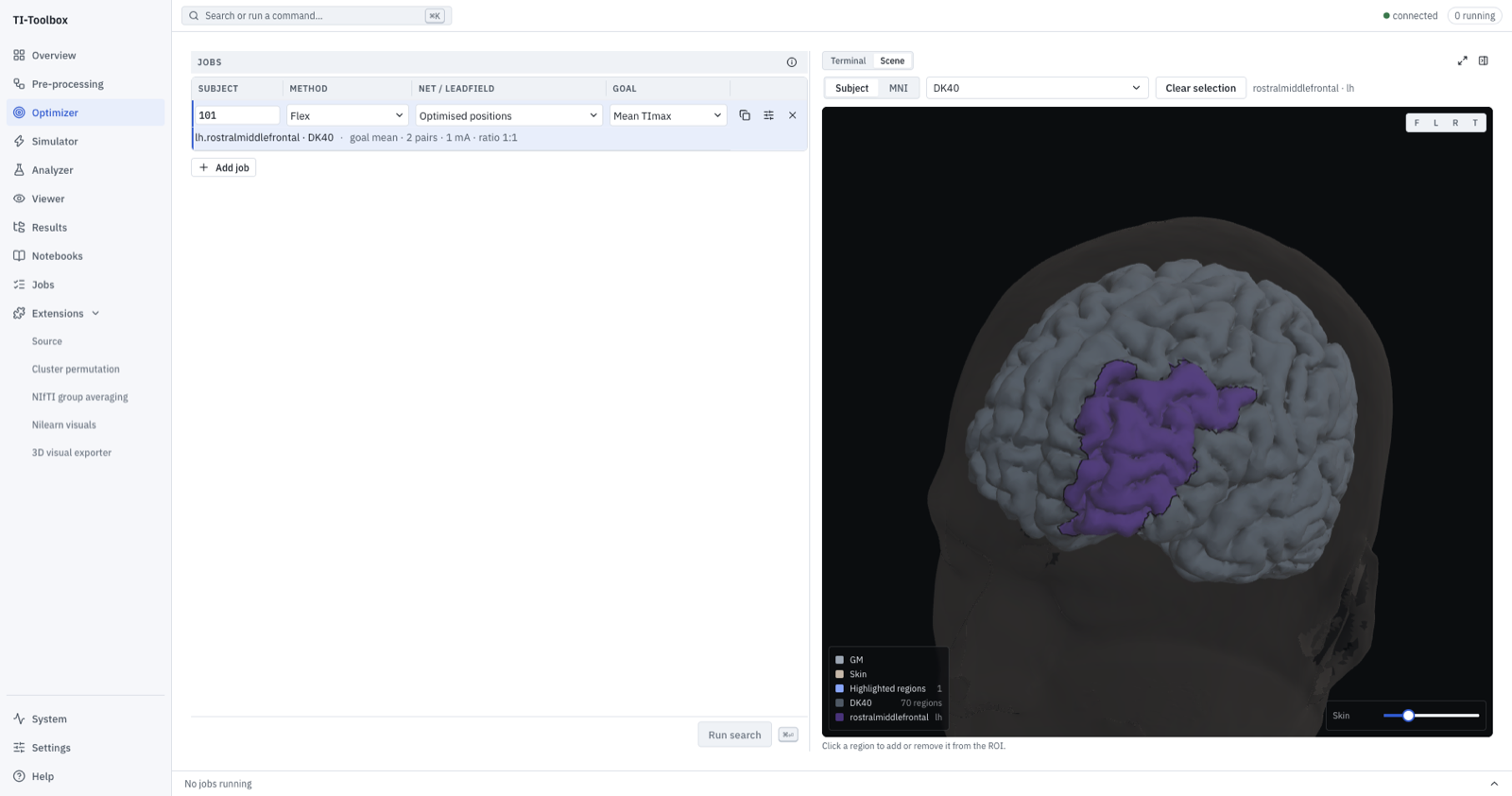The Optimizer. Flex is a method in a job row, not a page of its own; the atlas in the pane is the ROI you are choosing.

The interface provides comprehensive controls for:

• Basic Parameters: Subject selection, optimization goal, and post-processing method
• Electrode Parameters: Radius and current settings
• ROI Definition: A shared ROI picker with four modes – Cortical, Subcortical, Spherical, and NIfTI mask – used for both the ROI and the optional non-ROI; see Defining the ROI below
• Stability Options: Iteration limits, population size, and CPU utilization
• Mapping Options: EEG net electrode mapping capabilities

Defining the ROI

The ROI picker (desktop/src/renderer/pages/_shared/roi/, backed by tit/opt/roi_spec.py) is shared across flex-search, ex-search, and the analyzer. In flex-search it appears twice – once for the ROI, once for the optional “Specific Region” non-ROI described below – as a radio row with four modes:

• Cortical (default): pick regions from a FreeSurfer .annot atlas. An Atlas combo selects the parcellation, and the region selector opens a searchable finder that lists regions from both hemispheres by name. Selected regions become removable chips keyed by hemisphere-prefixed name (e.g. lh.precentral) – there is no separate hemisphere selector, so a single target can span both hemispheres from this one page.
• Subcortical: pick regions from a volumetric atlas. A Subject/MNI “Atlas Space” radio pair (Subject default) selects the coordinate space, a Tissue Type combo (GM / WM / GM+WM) sets the tissue restriction, and a Volume Atlas combo selects the atlas. the region selector adds selections keyed by integer label id.

• Spherical: a Subject/MNI coordinate-space radio pair (Subject default), a multi-row sphere table with X/Y/Z and radius in millimeters, an Add sphere button and a remove control on each row, and the 3-D pane beside the form for anatomical orientation. The guide is not the selected subject; enter coordinates in the explicitly selected coordinate space. A Volumetric checkbox enables a Tissue combo (GM / WM / GM+WM); unchecked, the sphere(s) are evaluated on the cortical surface instead.

• NIfTI mask: import a local .nii or .nii.gz file; it is copied into the project for the server. Positive voxels define the target; choose Subject or MNI space and the tissue restriction. Subject-space masks are used directly. MNI masks use the subject’s SimNIBS registration in m2m_<subject>/toMNI, with nearest-neighbor resampling to preserve the mask. The conformation affine alone is not an MNI registration.

For MNI atlases, the target pane’s Explode button pulls regions apart so deep structures can be clicked; see Atlases.

Whichever mode is used, the picker serializes to one of three dataclasses nested under FlexConfig. Every field on all three accepts either a single value or a list – a list unions several regions into one combined target: N spheres, cross-hemisphere cortical labels (e.g. lh.insula + rh.insula), or e.g. subcortical labels 17 and 53 for both hippocampi at once.

FlexConfig.SphericalROI

Field	Type	Default	Notes
x, y, z	float \| list[float]	required	Center coordinate(s) in mm; must be non-empty and of equal length
radius	float \| list[float]	10.0	Scalar (shared by every sphere) or one radius per center
use_mni	bool	False	Coordinates are in MNI space; SimNIBS transforms them to subject space during ROI setup
volumetric	bool	False	Evaluate on volume tetrahedra instead of the cortical surface
tissues	str	"GM"	"GM", "WM", or "both" – only used when volumetric=True

volumetric=False is the default, which evaluates the sphere on the cortical central surface, not a volume. For a deep target – amygdala, hippocampus, thalamus – this is an easy and consequential mistake: the sphere still picks up whatever surface vertices fall inside its radius, which for a subcortical center is the overlying cortex, not the target structure. Set volumetric=True for any target that is not on the cortical ribbon.

FlexConfig.AtlasROI

Field	Type	Default	Notes
atlas_path	str \| list[str]	required	Path(s) to .annot file(s); a scalar broadcasts to the number of labels
label	int \| list[int]	required	.annot label index/indices; must be non-empty
hemisphere	str \| list[str]	"lh"	"lh" or "rh", one per label

Always evaluated on the cortical central surface – AtlasROI has no tissues field. Because each label carries its own hemisphere and atlas path, a single AtlasROI can combine lh.insula and rh.insula (or regions from different atlases) into one union.

FlexConfig.SubcorticalROI

Field	Type	Default	Notes
atlas_path	str \| list[str]	required	Path(s) to volumetric atlas NIfTI file(s); a scalar broadcasts to the number of labels
label	int \| list[int] \| None	required	Integer label(s), or None for all positive voxels
tissues	str	"GM"	"GM", "WM", or "both" – applies to the whole union
atlas_space	str	"subject"	"subject" or "mni" – applies to the whole union

atlas_space="mni" targets one of the four bundled MNI atlases (see Atlases) instead of a subject-specific segmentation; SimNIBS transforms the selected label into subject space during ROI setup. A single tissues and atlas_space apply to every label in the union, and every atlas path is verified to exist before the run starts.

Python Example: Volumetric Union

from tit.opt import FlexConfig, run_flex_search

config = FlexConfig(
    subject_id="101",
    goal="mean",
    postproc="max_TI",
    current_mA=2.0,
    electrode=FlexConfig.ElectrodeConfig(),
    roi=FlexConfig.SubcorticalROI(
        atlas_path="/path/to/m2m_101/segmentation/aparc.DKTatlas+aseg.mgz",
        label=[17, 53],       # left + right hippocampus, unioned
        tissues="GM",
        atlas_space="subject",
    ),
)

result = run_flex_search(config)

For a deep spherical target, volumetric=True must be set explicitly, or the sphere silently falls back to the cortical-surface default described above:

roi = FlexConfig.SphericalROI(
    x=-25.0, y=-10.0, z=-20.0,
    radius=8.0,
    use_mni=True,
    volumetric=True,   # required for subcortical targets -- see note above
    tissues="GM",
)

Threshold-based focality

Choose Fixed, Adaptive, or Multi-threshold under Threshold-based focality. Fixed uses explicit field thresholds; Adaptive derives thresholds from an initial intensity search; Multi-threshold runs multiple threshold pairs. Existing configurations retain the pareto strategy value. These choices do not alter the threshold-free objective described below.

The focality optimization goal is a multi-objective function balancing ROI targeting with out-of-ROI field minimization:

Non-ROI Definition Methods

• Everything Else: Uses the complement of the ROI (everything outside the target region)
• Specific Region: Define a custom non-ROI using the same ROI picker (spherical, atlas, subcortical). Three constraints apply that are not obvious from the UI: the non-ROI picker is forced onto the same mode as the ROI picker – switching the ROI’s mode switches the non-ROI’s mode with it; the non-ROI’s spherical page has no Subject/MNI toggle, so non-ROI spheres are always subject-space even when the ROI itself is defined in MNI space; and the non-ROI’s own tissue selection is ignored – for volumetric spheres and subcortical atlases the non-ROI always inherits the ROI’s tissue compartment(s), not whatever its own Tissue control shows

Focality Thresholds - Critical for Optimization Success

As described in the original paper, focality optimization is fundamentally a constrained multi-objective problem where:

• Target Region (ROI): Field strength must exceed specified thresholds
• Avoidance Region (Non-ROI): Field strength must remain below specified thresholds
• Optimization Goal: Maximize field intensity in ROI while minimizing field spread outside ROI

Threshold Configuration Options

• Single Threshold: Binary classification where field must be below threshold in non-ROI and above threshold in ROI
• Dual Thresholds: Independent thresholds for each region, allowing asymmetric optimization constraints
• Derived Thresholds: thresholds always takes explicit numeric values – there is no in-loop adaptation. "dynamic"/"auto" are placeholders meaning “do not set a threshold; let SimNIBS use its own static default,” and the ROC-based objective path raises an error if no explicit numeric threshold is available. The workable pattern is an offline two-pass procedure: run a mean \(\mathrm{TI}_{\max}\) pass first, then derive the ROI/non-ROI thresholds from its field distribution and feed them into a focality run, as described below.

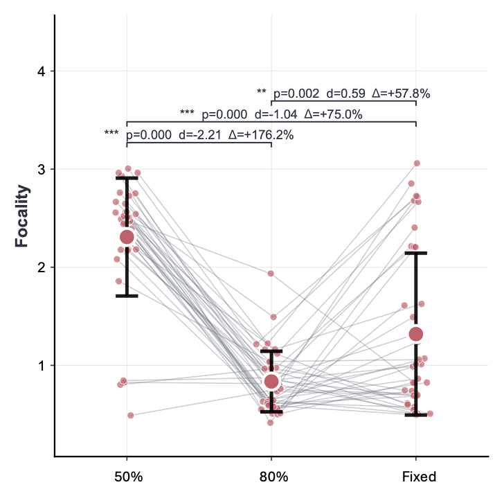
Focality optimization analysis: Comparative evaluation of threshold strategies reveals critical insights: threshold selection profoundly impacts results, with relative thresholds (50% of peak) yielding 75% higher focality than fixed thresholds, while 80% thresholds reduce focality by 37%, compared to fixed thresholds (0.1V/m and 0.3V/m) highlighting the importance of threshold optimization for precise neuromodulation. Dynamic % based thresholds were derived automatically from an intial pass of mean TImax search and applied to the upper bound only. The lower bound was kept at 20% from that value. Data regarding focality thresholds and optimization performance comes from the supplementary information of the TI-Toolbox reference.

Threshold-Free Focality Optimization

The focality_tf goal shares the broad aim of the ROC goal above, but uses a different scoring criterion – concentrate the field in the ROI and keep it out of the non-ROI – without asking the user to commit to a field threshold in advance. Instead of counting elements above and below a cutoff, it scores the ratio of the mean ROI field to the mean non-ROI field:

\[\texttt{focality\_tf} = \frac{\operatorname{mean}\!\left( E_{\mathrm{ROI}} \right)^{\,1+w}} {\operatorname{mean}\!\left( E_{\text{non-ROI}} \right)}\]

Larger is better; the optimizer minimizes its negative. Both means use the samples in the declared regions. Non-ROI is the declared comparison region: it can be the ROI complement or a separately specified region; it is not automatically every sample outside the ROI. This mean ratio does not constrain individual off-target hot spots; the non-ROI 95th percentile remains a separate diagnostic.

The Intensity Weight

The exponent \(w\) is the intensity_weight parameter (range \([0, 1]\), default 0.0) and controls the trade-off between focality and on-target strength:

• intensity_weight = 0.0 – pure focality ratio, with no absolute intensity preference. Scaling both regions equally leaves the score unchanged. This is the default.
• intensity_weight = 1.0 – intensity-weighted focality. The ROI mean is squared; the non-ROI mean still penalizes spread. This is not the intensity-only Mean TImax objective.
• Intermediate values interpolate between the two.

Why Threshold-Free Matters

The ROC goal depends on user-selected thresholds. It minimizes the distance from ideal ROI coverage above the ROI threshold and zero non-ROI coverage above the non-ROI threshold. These are scoring targets, not enforced constraints. Poorly chosen thresholds can make many candidates have identical coverage and therefore identical scores. An infeasible threshold pair does not imply that every candidate ties: partial coverage can still distinguish candidates. Solver termination does not establish that the requested thresholds were attained.

focality_tf avoids choosing threshold pairs. It can still assign equal scores to different candidates, and mesh discretization can create flat regions. Neither a finite contrast nor a solver stopping proves convergence, a global optimum, or useful target intensity. Nonfinite, signed-negative, empty, or numerically degenerate non-ROI values are rejected rather than rewarded with an inflated ratio.

Historical study below: these measurements used the earlier p95-denominator focality_tf, except for the explicitly named intensity-weighted mean-ratio arm. They are preserved as historical evidence, not validation measurements of the corrected mean-denominator objective.

That does not make it failure-proof, though – a scale-free ratio objective trades one failure mode for a different one. Because it scores separation, not dose, it can rate a candidate highly for being cleanly separated from the non-ROI even when almost no field reached the target at all. In the mini-study below, a threshold-free direct-AUC run scored AUC 0.931 on just 0.047 V/m of on-target field, and focality_tf itself bottomed out at 0.084 V/m in its worst cell. Always read a focality or AUC score next to the ROI-mean field it was computed on.

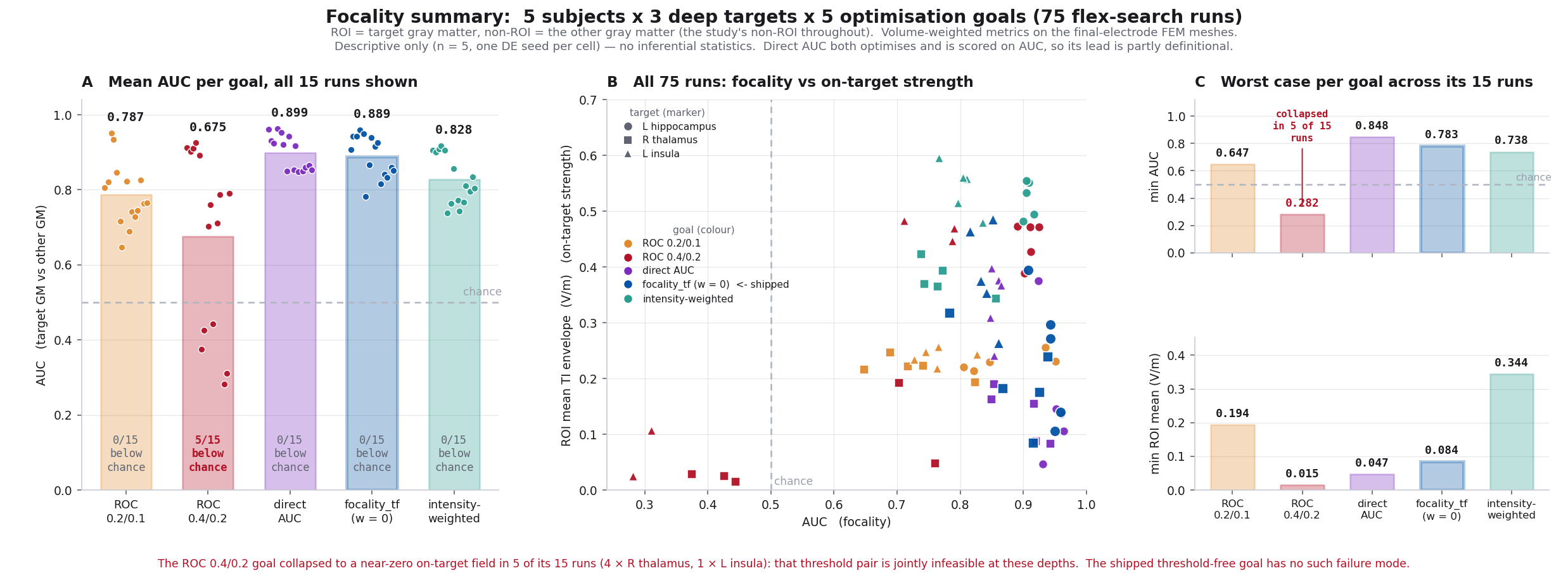
Summary across all 75 flex-search runs (5 subjects x 3 deep atlas targets x 5 optimization goals): mean AUC per goal, the focality-vs-on-target-strength tradeoff for every run, and each goal’s worst-case AUC and worst-case ROI field strength. On average across the 15 subject-target cells, the threshold-free objectives outperformed both ROC threshold settings on focality (AUC); focality_tf (the historical p95 goal, w = 0) beat both ROC arms in 13 of 15 cells (86.7%), losing only at sub-101 and sub-103 L-hippocampus – the one target where the aggressive threshold pair (0.4/0.2 V/m) turned out to be feasible. That same aggressive ROC goal failed outright where its threshold pair was jointly infeasible at depth: it scored below chance (AUC < 0.5) in 5 of its 15 cells, and collapsed to near-zero on-target field – a separate, dose-based criterion – in 6. focality_tf had no failures under either criterion. This does not make focality obsolete – where a defensible and attainable threshold exists, it optimizes precisely the criterion the user cares about – but it does mean the threshold has to be validated for the target at hand.

When to Use Which

	focality (ROC)	focality_tf (threshold-free)
Thresholds required	Yes – thresholds must be set	No
What is scored	ROC separation of ROI and non-ROI elements at the chosen cutoff	mean ROI field raised to 1 + intensity_weight, divided by mean non-ROI field
Behavior at deep targets	Can have flat scores when candidates have identical threshold coverage	Avoids fixed thresholds; ties and flat regions remain possible
Intensity trade-off	Implicit in the threshold choice	Explicit via intensity_weight
Use when	You have a threshold you can defend and that the target can actually reach – e.g. derived from a prior mean \(\mathrm{TI}_{\max}\) pass	You do not want to commit to a threshold up front, or the target is deep enough that feasibility is in doubt
Worst case over 15 subject-target cells*	Min AUC 0.282; min ROI mean 0.015 V/m	Min AUC 0.783; min ROI mean 0.084 V/m
Dose guarantee	Not guaranteed – always check ROI mean	Not guaranteed – always check ROI mean

* Historical p95-denominator results, not a benchmark of the current mean-denominator objective. From the mini-study below; the focality column here is specifically the aggressive thresholds=0.4,0.2 V/m arm – a different threshold choice will perform differently.

Both goals use the same ROI and non-ROI setup, so switching between them requires no change to the region definitions. One restriction applies only to focality_tf: it cannot be run with detailed_results=True (see Detailed Results).

Caveats

Read every number in this section with these in mind:

• n = 5 subjects, descriptive only. No inferential statistics were run – no p-values, no confidence intervals, no multiple-comparison correction.
• One DE seed per cell. Run-to-run optimizer variability was not characterized, so differences of roughly 0.02-0.05 AUC are within plausible seed noise. The 0.899 vs. 0.889 AUC gap between direct AUC and focality_tf in the table below is not a demonstrated real difference on that basis alone.
• Direct-AUC’s lead is partly definitional. AUC is both its optimization objective and the evaluation metric used to score all five goals here, so treat its AUC column as a ceiling reference, not an independent win.
• The non-ROI is all other gray matter, not the whole brain. The study used SubcorticalROI(tissues="GM"), and SimNIBS’s everything_else non-ROI inherits that tissue restriction – white matter and CSF were never part of the non-ROI in any run.
• Statistics are volume-weighted, computed on the final-electrode FEM meshes rather than the optimizer’s mid-search arrays. This changes how the summary statistics are computed, not which tissue is included, and the ranking of the five goals is unchanged versus unweighted means.
• Three deep targets only – hippocampus, thalamus, insula. Nothing here speaks to superficial cortical targets, where the ROC thresholds are far more likely to be jointly feasible.
• AUC is scale-free. It measures separation, not dose. Never read an AUC value without the ROI-mean field next to it.

Pooled results (n = 15 subject-target cells per goal)

Goal	AUC	ROI mean (V/m)	non-ROI mean (V/m)	Focality ratio	Off-target vol >=0.2 V/m (%)	tf score
focality (ROC 0.2/0.1 V/m)	0.787 ± 0.084	0.230 ± 0.018	0.143 ± 0.039	1.713 ± 0.460	21.2 ± 11.2	0.706 ± 0.194
focality (ROC 0.4/0.2 V/m)	0.675 ± 0.239	0.272 ± 0.208	0.152 ± 0.093	1.497 ± 0.627	24.0 ± 20.1	0.686 ± 0.254
threshold-free: direct AUC	0.899 ± 0.046	0.212 ± 0.122	0.119 ± 0.069	1.815 ± 0.268	15.2 ± 21.2	1.037 ± 0.096
focality_tf (w = 0) – shipped	0.889 ± 0.056	0.276 ± 0.124	0.159 ± 0.075	1.776 ± 0.255	27.8 ± 29.0	1.051 ± 0.088
threshold-free: intensity-weighted	0.828 ± 0.066	0.481 ± 0.083	0.301 ± 0.053	1.632 ± 0.356	74.7 ± 16.4	0.846 ± 0.093

Historical formula distinction: the intensity-weighted study arm used mean(ROI)^2 / mean(non-ROI), the algebraic form now used at intensity_weight = 1. The study’s focality_tf arms instead used a p95 denominator. Those historical arm labels and measured values have not been recomputed; they do not establish convergence or performance for the current implementation.

Reliability

focality (ROC 0.4/0.2 V/m) has a pooled AUC standard deviation of ±0.239 – four to five times either threshold-free ranking goal’s (±0.046 for direct AUC, ±0.056 for focality_tf). The aggressive ROC goal is not uniformly bad, it is unreliable: its outcome depends heavily on whether its fixed thresholds happen to be feasible for the subject and target at hand.

Failures

Five of the 75 runs (6.7%) scored AUC below 0.5 – worse than chance separation – and all five are the aggressive focality (ROC 0.4/0.2 V/m) goal: 3 at R-thalamus, 2 at L-insula, 0 at L-hippocampus. Neither threshold-free goal (direct AUC, focality_tf) had a single run below chance.

A separate, dose-based flag counts runs whose ROI mean fell below one third of that target’s median ROI mean across all goals and subjects – catching cases where the AUC looks acceptable but almost no field reached the target. By goal: focality (ROC 0.4/0.2 V/m) = 6, threshold-free direct AUC = 1, focality (ROC 0.2/0.1 V/m) = 0, focality_tf (w = 0) = 0, threshold-free intensity-weighted = 0. Neither criterion alone catches everything: sub-106 R-thalamus under ROC 0.4/0.2 scored AUC 0.760 (above chance) while delivering only 0.048 V/m on target – caught by the dose flag but not by the below-chance criterion.

Depth dependence

The aggressive focality (ROC 0.4/0.2 V/m) goal performs best, among its own three targets, at L-hippocampus (AUC 0.908 ± 0.013, ROI mean 0.447 ± 0.037 V/m – the second-highest ROI mean of any goal at that target) and worst at R-thalamus (AUC 0.541 ± 0.177) and L-insula (AUC 0.576 ± 0.258). The same 0.4/0.2 V/m threshold pair happens to be feasible at hippocampus depth and infeasible at the other two – and the goal gives the user no warning about which case they are in before the run finishes.

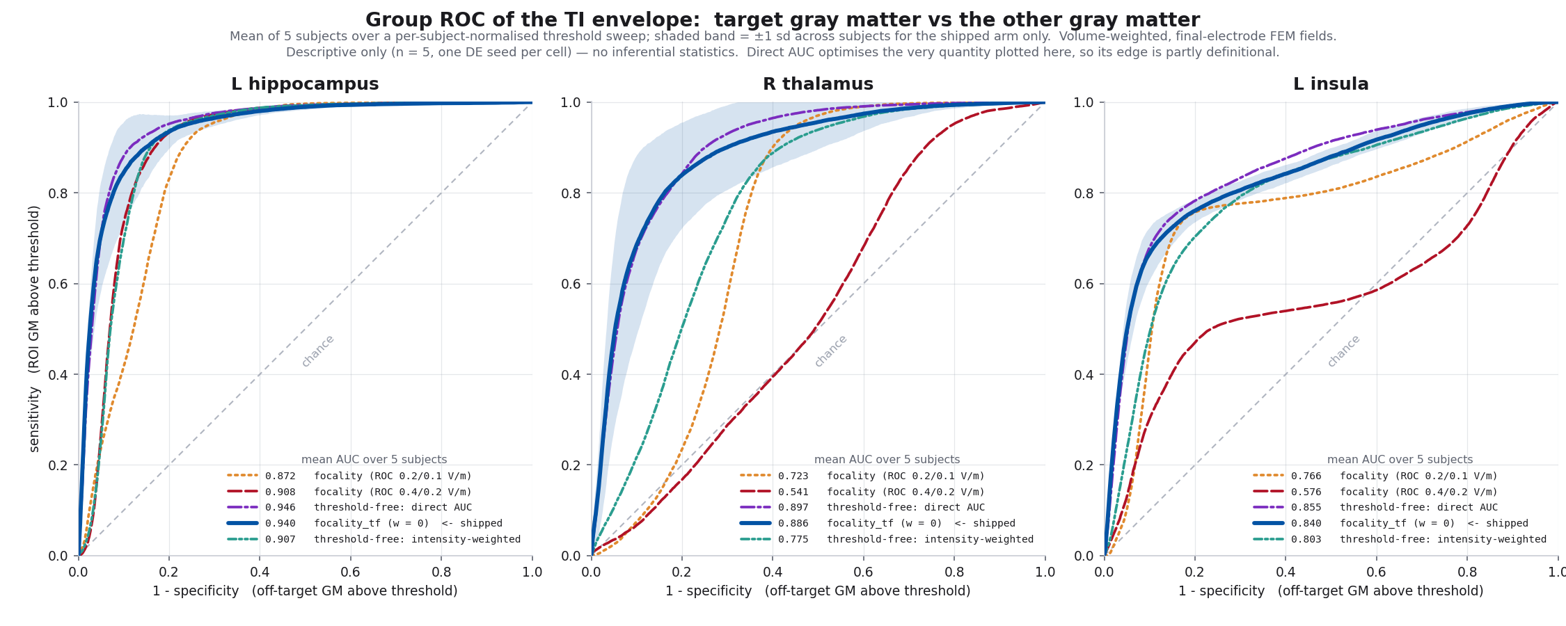
Group ROC curves of the TI envelope (target gray matter vs. the other gray matter) for each of the three deep targets, comparing all five optimization goals by mean AUC over the 5 subjects; the shaded band shows ±1 SD across subjects for the historical p95 focality_tf (w = 0) arm only. AUC drops sharply for the ROC threshold goals at R-thalamus and L-insula, while the threshold-free goals (direct AUC, focality_tf, intensity-weighted) stay high across all three targets.

Worst case

The shipped goal’s worst run across all 15 cells, AUC 0.783, essentially matches the milder ROC goal’s average (0.787 ± 0.084). The aggressive ROC goal’s worst run drops to AUC 0.282 (sub-103, L-insula); the lowest on-target field reached by that same goal anywhere in the study is 0.015 V/m (sub-107, R-thalamus) – two separate worst-case runs, not necessarily the same one.

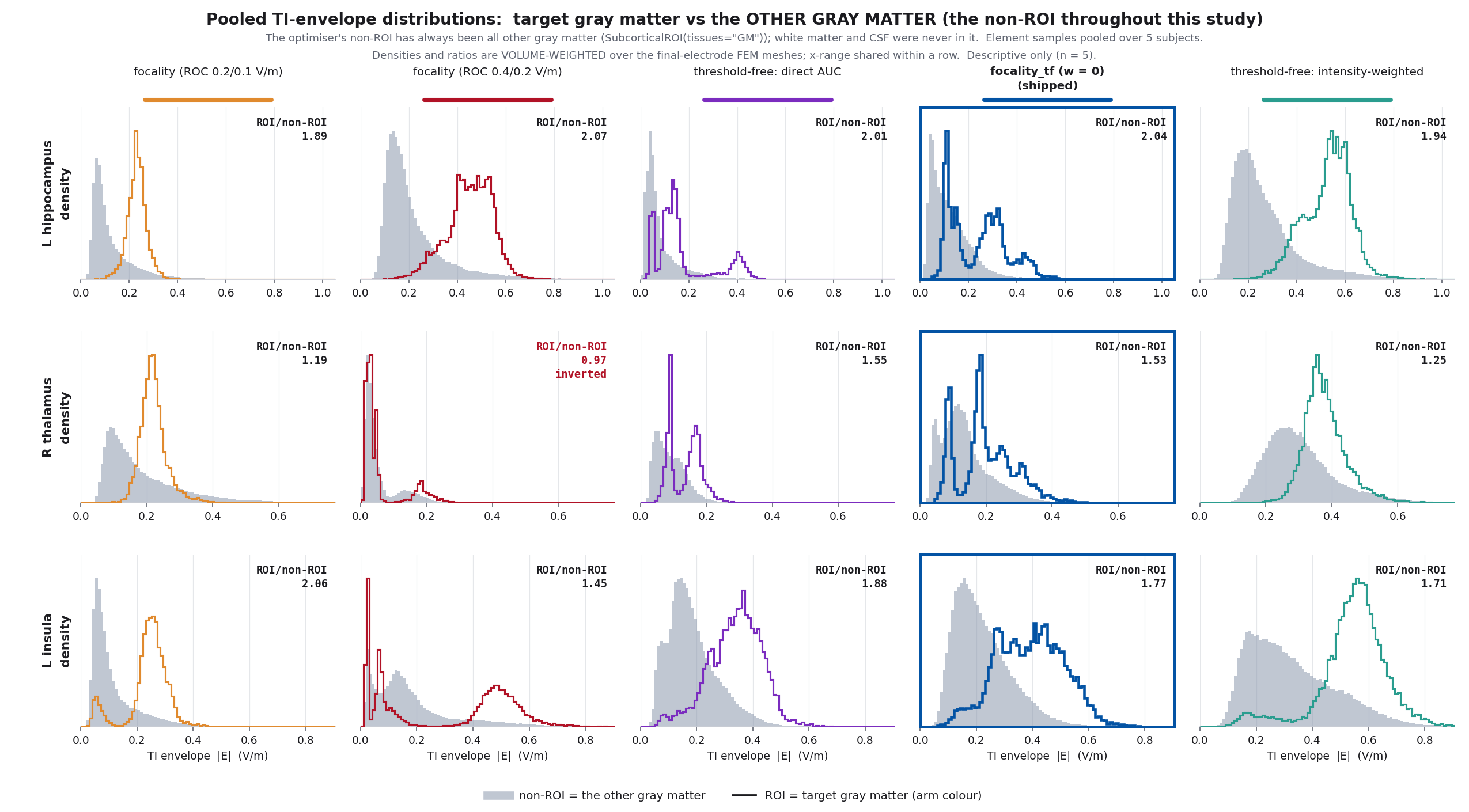
Pooled, volume-weighted TI envelope field-strength distributions (target gray matter vs. the other gray matter), element samples pooled over the 5 subjects, shown as a 3-target x 5-goal grid with the group ROI/non-ROI mean ratio annotated in each panel. At R-thalamus, the ROC 0.4/0.2 goal’s ROI/non-ROI ratio inverts – the pooled group ratio annotated in the figure is 0.97, and the per-subject mean for that cell is 0.975 +/- 0.267 – meaning the off-target gray matter received, on average, slightly more field than the target. This is consistent with the near-zero on-target fields shown in the summary figure above.

Current-Ratio Optimization

By default the two TI channels carry equal current. The optimize_current_ratio flag opts into searching that split as well: the total injected current is held constant and divided between the two channels, with ratio_levels (default 21) setting the density of the grid, which spans 1:3 to 3:1. The total defaults to 2 x current_mA and can be set explicitly with ratio_total_mA.

What Each Channel Carries

Holding the total fixed means the per-channel current necessarily moves. Over the 1:3 to 3:1 grid each channel spans a quarter to three quarters of the total – that is, 0.5x to 1.5x the configured current_mA (the Optimizer’s Electrode Current). With the default total of 2 x current_mA and current_mA = 2.0, a channel is driven anywhere between 1.0 mA and 3.0 mA, with the pair always summing to 4.0 mA. current_mA is therefore the center of the searched range, not a per-channel ceiling: choose it (or set ratio_total_mA directly) so that the 1.5x end is still within the dose you intend to deliver.

The grid always contains the balanced 1:1 split – ratio_levels is rounded up to the next odd number so the midpoint of the sweep is the exact even split. The grid includes the equal-current split for each fixed placement. This does not guarantee a better final placement from a finite stochastic search.

That guarantee is about the objective value only. It is not a guarantee about the delivered field: under a focality-only objective with a tight off-target bound, the optimizer can pick an extreme split simply to turn the whole field down, since a weaker envelope is an easy way to satisfy a hard cap on off-target field. Measured on sub-101 L-hippocampus at a fixed 4 mA total, holding electrode positions fixed and varying only the split: 1:3 gives 0.185 V/m on target (focality ratio 1.64, attenuated); 2:2 gives 0.361 V/m (focality ratio 1.92, best on both); 3:1 gives 0.196 V/m (focality ratio 1.16, attenuated). Focality peaks near 1:1 in this example and drops off toward both extremes – the extreme splits attenuate the whole field rather than sharpening it.

Why the Split Matters

The TI envelope amplitude is capped by the weaker of the two channels – for co-linear fields the modulation depth is \(2 \min\!\left( \lVert \mathbf{E}_1 \rVert, \lVert \mathbf{E}_2 \rVert \right)\). The split therefore does two things at once: it scales the envelope, because the ceiling moves with the weaker channel, and it steers it, because the locus where the two channels balance shifts toward the weaker one. Because the FEM is linear, a per-channel rescale is enough to evaluate any split without a new solve (Lee et al. 2022). Published TI optima are rarely the 1:1 split that flex-search fixes by default (Lee et al. 2020; Inoue et al. 2025, n = 60), so leaving the split fixed gives up a free axis of the search space.

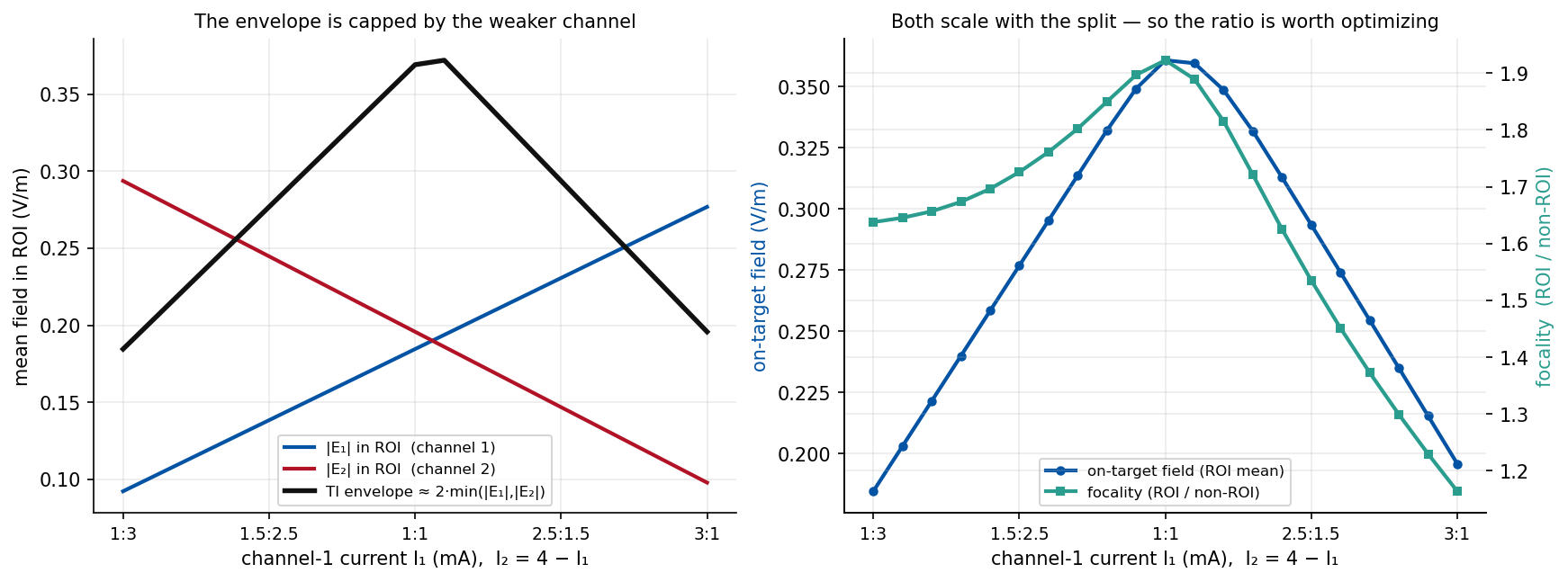
How the two-channel current split scales and steers the TI envelope. Because the envelope is bounded by the weaker channel, an unequal split trades peak amplitude against the position of the interference locus. This particular montage was itself optimized at 1:1, so 1:1 is near-optimal for it by construction – post-hoc ratio tuning on top of an already-1:1-optimized placement gains only about +0.8% here. The payoff from a free ratio comes from searching it jointly with electrode placement (below), which can reach placements a 1:1-constrained search would never consider in the first place.

Calibrating the Off-Target Bound

The trap described above only bites when a focality objective’s off-target bound is tight enough to be binding well away from the 1:1 split. The fix is to calibrate the bound against what the target can actually achieve rather than picking a number in isolation: sweep the bound across the field’s achievable range and check whether the optimizer’s chosen split still moves as a result. On a single subject (101), the achievable off-target RMS field ranged:

Target	Achievable off-target RMS (V/m)	Sensible bound sweep
L-hippocampus	0.065 - 0.316	0.05 … 0.38
R-thalamus	0.041 - 0.353	0.03 … 0.42
L-insula	0.152 - 0.436	0.12 … 0.52

These ranges are from a single subject and from a reduced-budget sweep (maxiter=4, popsize=6, well under the SimNIBS default of maxiter=1000, popsize=13), so the front they trace is under-converged. Treat them as a starting point for calibrating a bound on a new subject, not as a target’s true achievable range.

Searched Jointly, Not Afterwards

The ratio is optimized jointly with electrode placement, not applied as a post-hoc refinement. Every candidate placement is scored at its own best split, so the optimizer sees the landscape it will actually be evaluated on. Running a ratio sweep after the fact would only refine a montage that had already been selected under a 1:1 assumption – a different, and worse, optimum.

The joint search adds envelope and reduction work. The FEM is linear, so for a fixed electrode placement the per-channel fields simply scale with the injected current: evaluating an additional split is a rescale of the already-computed fields and a re-combination of the envelope, with no new FEM solve. Candidate splits are ranked on a deterministic subsample of the non-ROI, and only the winning split is re-scored on the full non-ROI, so the several-million-element non-ROI is traversed once per evaluation rather than once per split.

Current-ratio optimization works with any goal (mean, max, focality, focality_tf). The winning split is applied to the final electrode simulation, so the fields written to disk are the ones the objective actually scored, and it is recorded in the run manifest (flex_meta.json).

Python Usage

from tit.opt import FlexConfig, run_flex_search

config = FlexConfig(
    subject_id="101",
    goal="focality_tf",           # threshold-free focality
    postproc="max_TI",
    current_mA=2.0,
    intensity_weight=0.0,         # 0 = balanced, 1 = intensity-first
    electrode=FlexConfig.ElectrodeConfig(
        shape="ellipse",
        dimensions=[8.0, 8.0],
        gel_thickness=4.0,
    ),
    roi=FlexConfig.SphericalROI(
        x=-35.0, y=5.0, z=5.0,
        radius=10.0,
        use_mni=True,
    ),
    non_roi_method="everything_else",
    optimize_current_ratio=True,  # search the channel split jointly
    ratio_total_mA=4.0,           # defaults to 2 * current_mA
    ratio_levels=21,              # grid density, spanning 1:3 .. 3:1
)

result = run_flex_search(config)
print(f"Best value: {result.best_value:.4f}")

Note that thresholds is not used by focality_tf and can be omitted; it remains required for the ROC-based focality goal.

Reviewing evaluated candidates

Open a completed run in Results → Evaluated candidates. Expand the preview pane for a side-by-side table and plot. The plot defaults to ROI mean intensity versus recorded focality; select a row or a point to highlight the same candidate and update the existing montage preview. Selecting a point on another table page brings that row into view. Use in Simulator creates an editable draft of that candidate; nothing runs automatically.

The plot loads up to 10,000 recorded candidates in the selected sort order, independently of the table page. The table still pages through the full history. Loading, incomplete history, and missing measurements are shown explicitly. Outlined points form the frontier among the loaded comparable evaluations, not all possible montages or a guaranteed global Pareto front. Historical p95-based ratios retain their own label. Read intensity alongside focality; a high ratio can still have a weak target field.

Flex records valid trials under candidate_history, with scalar CSV metrics, full-precision geometry and a manifest describing the objective and stopping reason. Invalid placements are counted separately. Older runs retain their saved winner but have no fabricated trial history. Missing measurements are shown as unavailable. Intensity-only non-ROI measurements are opt-in because they add processing cost; threshold-free focality already evaluates its declared non-ROI.

Flex metrics use unweighted samples from their declared regions. Ex’s recorded whole-gray-matter mean includes the target, so it is not the same region definition. Ex replay also uses recorded CSV precision and editable Simulator electrode defaults because historical CSVs do not contain physical electrode dimensions. Final remeshed simulation fields may differ from optimization estimates.

Detailed Results

For callable or current-ratio objectives, MATLAB configuration export is deliberately omitted with a log message: SciPy cannot preserve the Python scoring function. Use the JSON configuration and candidate manifest; an empty MATLAB goal is not a reproducible objective. Native string goals still support MATLAB export.

detailed_results=True cannot be combined with the current-ratio search or with the focality_tf goal. Both install a Python callable as the optimization goal, and SimNIBS cannot serialize a callable into its detailed-results HDF5 file, so requesting the combination raises an error before the run starts rather than failing partway through. Leave detailed_results at its default of False – the GUI does not expose it – and read run metadata from flex_meta.json instead.

Multi-Start Optimization

Flex Search supports multiple starts to explore different initial conditions and retain the best valid evaluated solution. This can improve coverage but does not guarantee convergence:

• Multiple Runs: Configure the number of optimization runs (default: 1, recommended: 3-5 for critical applications)
• Best Solution Selection: Automatically selects the optimization run with the lowest function value
• Comprehensive Reporting: Generates multi-start summary files with run-by-run analysis

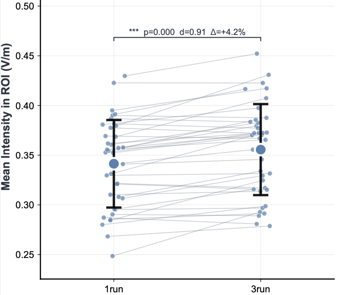
Multi-start optimization validation: Analysis demonstrates that running multiple independent optimizations with different random seeds yields superior solutions compared to single runs; 4.18% improvement in mean TImax. While statistically significant, the modest gains should be weighed against the increased computational cost. Data regarding multi-start optimization performance comes from the supplementary information of the TI-Toolbox reference.

Electrode Mapping and Target Accessibility

The transition from unconstrained optimization solutions to practical electrode montages represents a critical step in clinical translation. While genetic algorithms can identify theoretically optimal electrode positions anywhere on the scalp, its transition to clinical application may be difficult. Our electrode mapping algorithm bridges this gap by finding the best approximation of optimized positions using available electrode sites. For this study, we utilized the inner 185 electrodes of the GSN-HydroCel-256 system (EGI/Philips), which provides high-density coverage. A combinatorial optimization method that solves the assignment problem in polynomial time. By minimizing the total Euclidean distance between optimized and standard positions, this approach ensures good representation of the intended field distribution while maintaining practical feasibility.

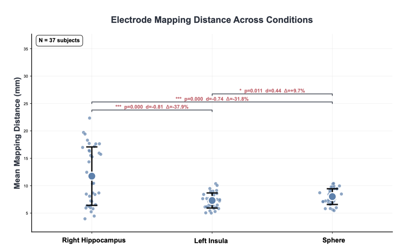
Electrode mapping challenges: Analysis of optimized electrode positions reveals depth-dependent mapping distances across anatomical targets, with subcortical structures like the hippocampus requiring significantly larger electrode separations (11.74 ± 5.33 mm) compared to cortical regions like the insula (7.30 ± 1.38 mm) or spherical ROIs (8.01 ± 1.43 mm). This pattern reflects the fundamental challenge of targeting deep brain structures with scalp electrodes, where optimal montages often requires large distances between electrodes which may be positioned on the lower scalp that does not have dense electrode coverage. Data regarding electrode mapping distances comes from the supplementary information of the TI-Toolbox reference.

Report

Every run writes a flex-search report: the target with the run’s own target figure, what the score means, the optimised electrode centres in subject coordinates with the valid-scalp figure, the dose, and one row per optimiser run. It draws no EEG cap and names no cap electrodes, because flex-search positions are free; mapped EEG-net labels, when mapping is enabled, are in electrode_mapping_<net>.json. See Reports.

Output Manifest (flex_meta.json)

Every flex-search run writes a flex_meta.json file to the output folder. This manifest is the single source of truth for run metadata – downstream consumers (simulator tab, GUI) read this instead of parsing folder names.

The manifest contains:

• Run configuration (goal, postproc, electrode, ROI, anisotropy)
• Result summary (success, best value, all function values)
• Timestamps and labels for display

Advanced Features

Anisotropy Support

Flex-search passes anisotropy parameters directly to SimNIBS, enabling optimization with direction-dependent tissue conductivity. The anisotropy_type parameter accepts four models:

Type	Description
scalar	Isotropic, piecewise-constant conductivity (default)
vn	Volume-normalized anisotropic tensors
dir	Direct linear rescaling of diffusion tensor eigenvalues
mc	Mean conductivity (isotropic but spatially varying)

Additional parameters aniso_maxratio (default: 10.0) and aniso_maxcond (default: 2.0) control the anisotropy bounds.

Valid Skin Region Validation

Flex-search optimization is constrained to valid skin regions where electrodes can be safely placed. The green region represents the valid skin area for electrode placement during optimization, while red “x” marks indicate HD-EEG electrodes that fall outside this valid region.

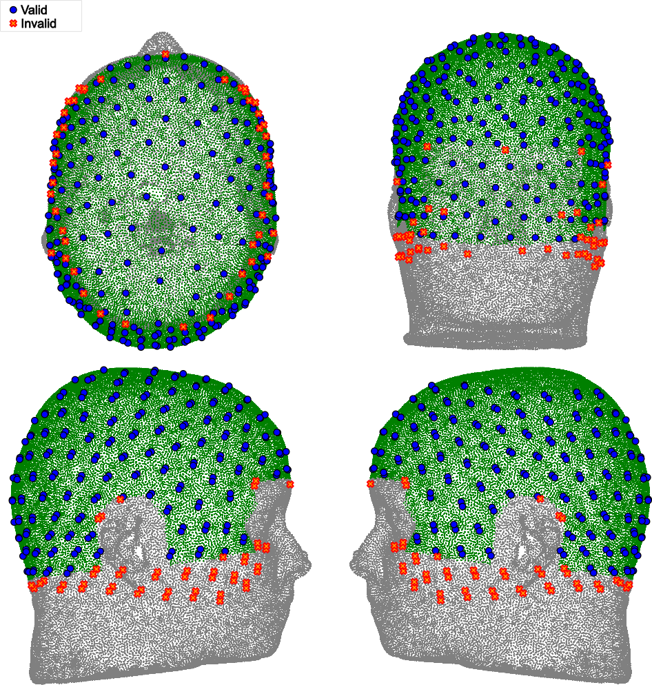
If electrode positions fall outside the valid skin region, the valid skin region can be manipulated through preprocessing, or ex-search can be used as an alternative since it is not constrained by skin region limitations.

Valid Skin Region Margin

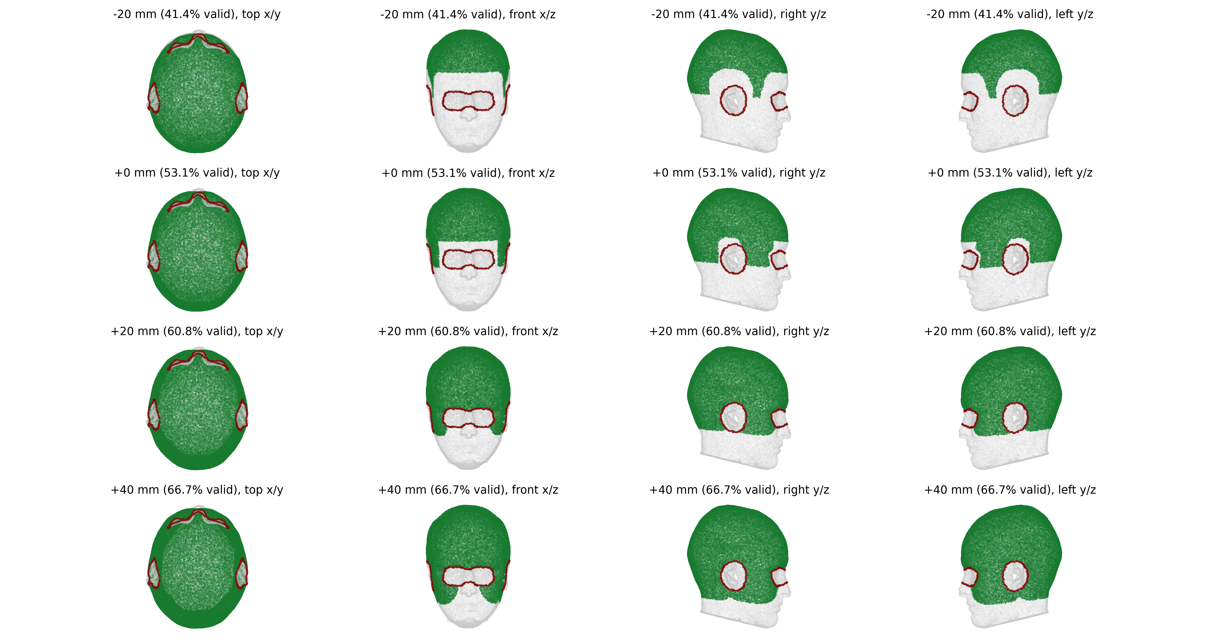
The flex-search skin constraint can be adjusted directly from scripts or from the GUI. skin_region_margin_mm applies a signed millimeter margin to the default SimNIBS valid skin region: negative values constrict the region, positive values expand it. The default is 0.0, which preserves the standard SimNIBS mask.

For positive margins, avoid_landmark_regions=True keeps fiducial-derived ear and orbital exclusion zones invalid. This guard uses scalp landmarks only (Nz, LPA, and RPA) and does not depend on eye tissue labels.

Target preview

The Scene pane follows the active job. Cortical regions remain clickable; masks, subcortical regions and spheres show a read-only target extent in subject space. Edit these targets in the job form. The preview shows geometry before search-specific tissue and mesh filtering.

Additional result examples

These captures predate the v3 Optimizer layout, but the scientific outputs remain useful examples. They are not instructions for the current interface.

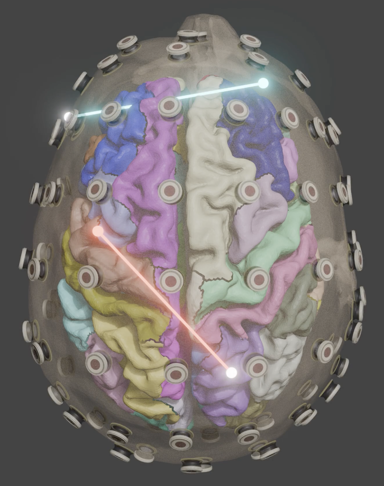Evolutionary optimization can place electrodes continuously on the valid scalp rather than restricting them to an EEG net.

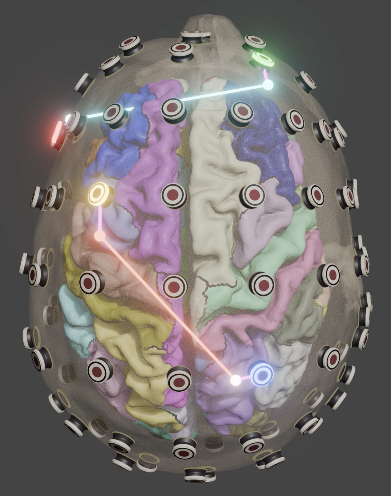The mapping step assigns optimized positions to the nearest feasible, distinct EEG-net sites.

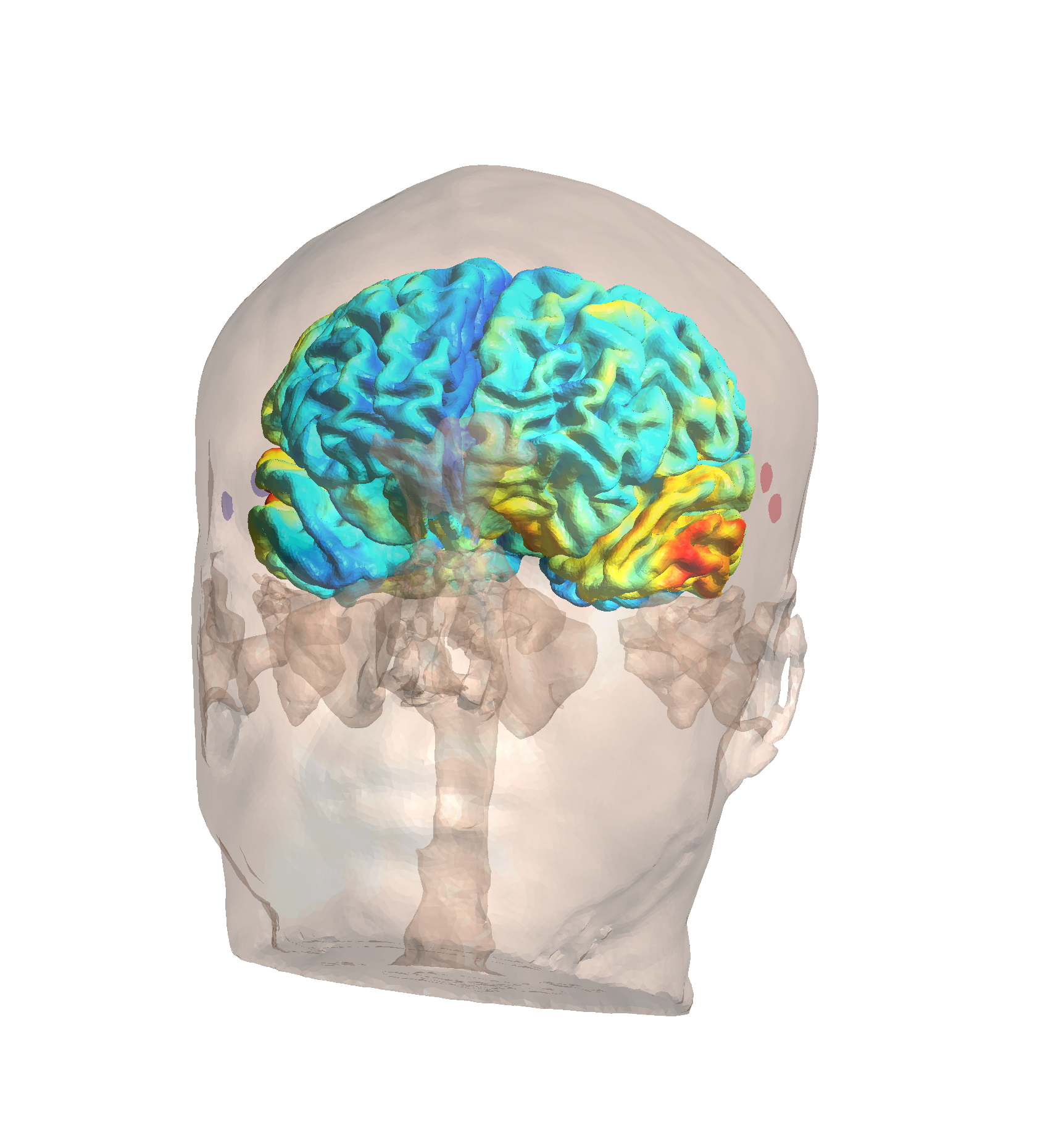The optimized TI_max field over the cortical surface.

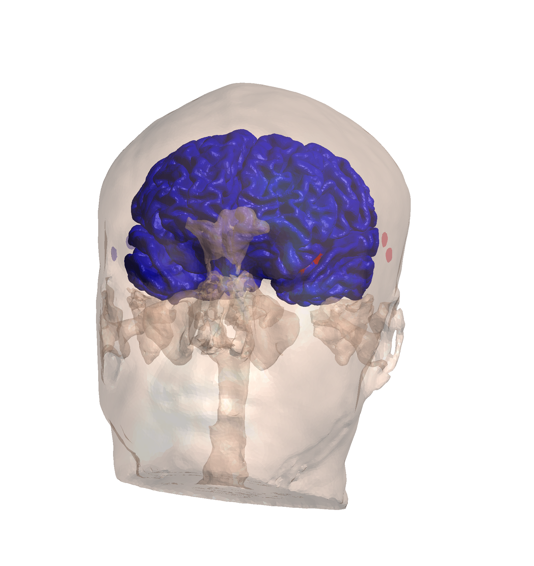The same maximum-envelope field restricted to the target ROI.

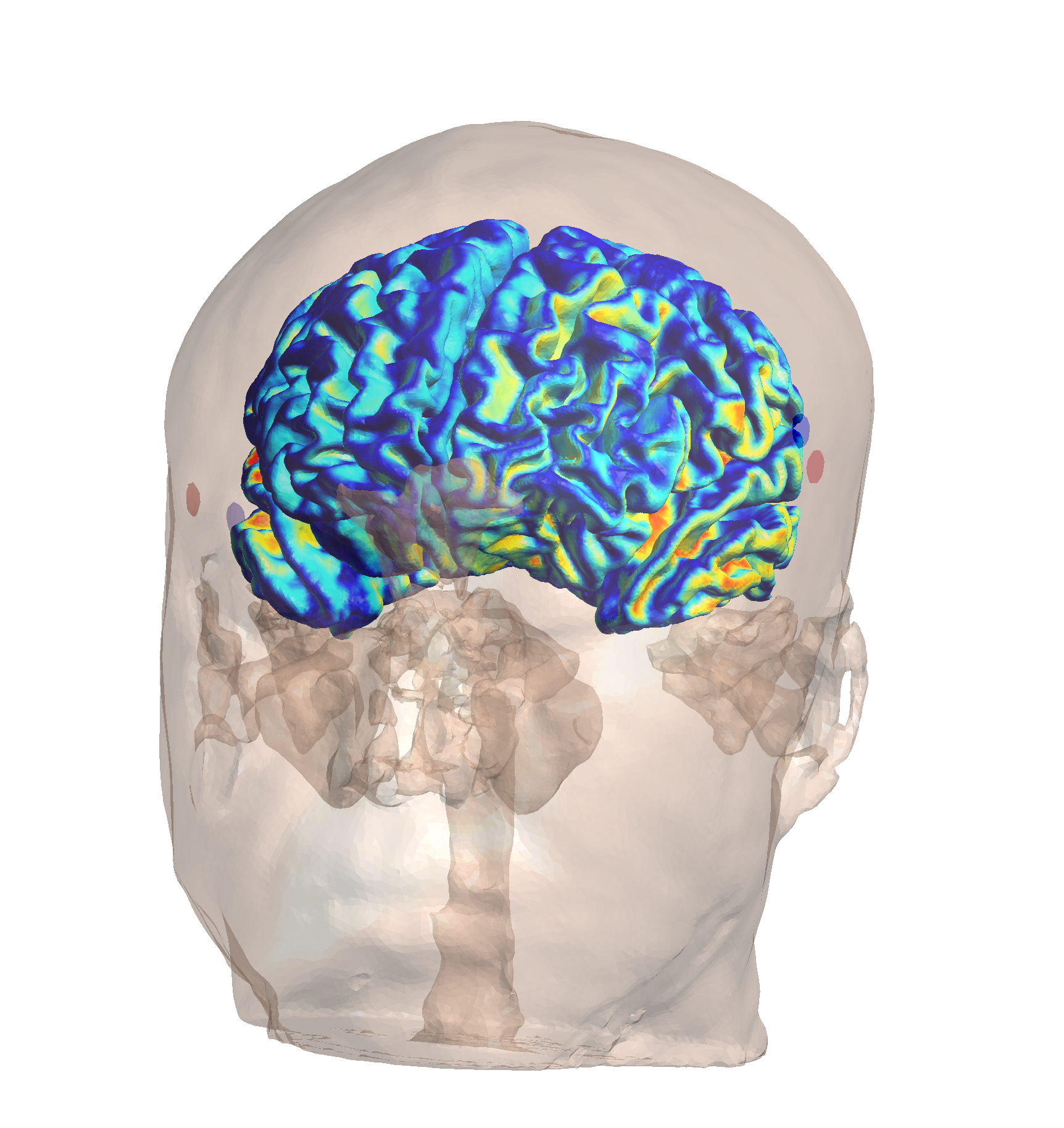The field component normal to the cortical surface.

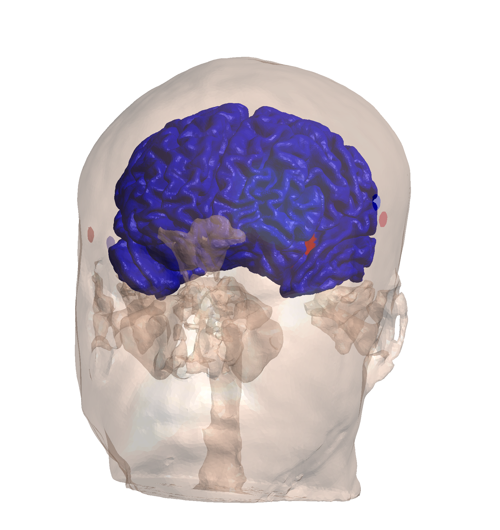The normal component restricted to the target ROI.

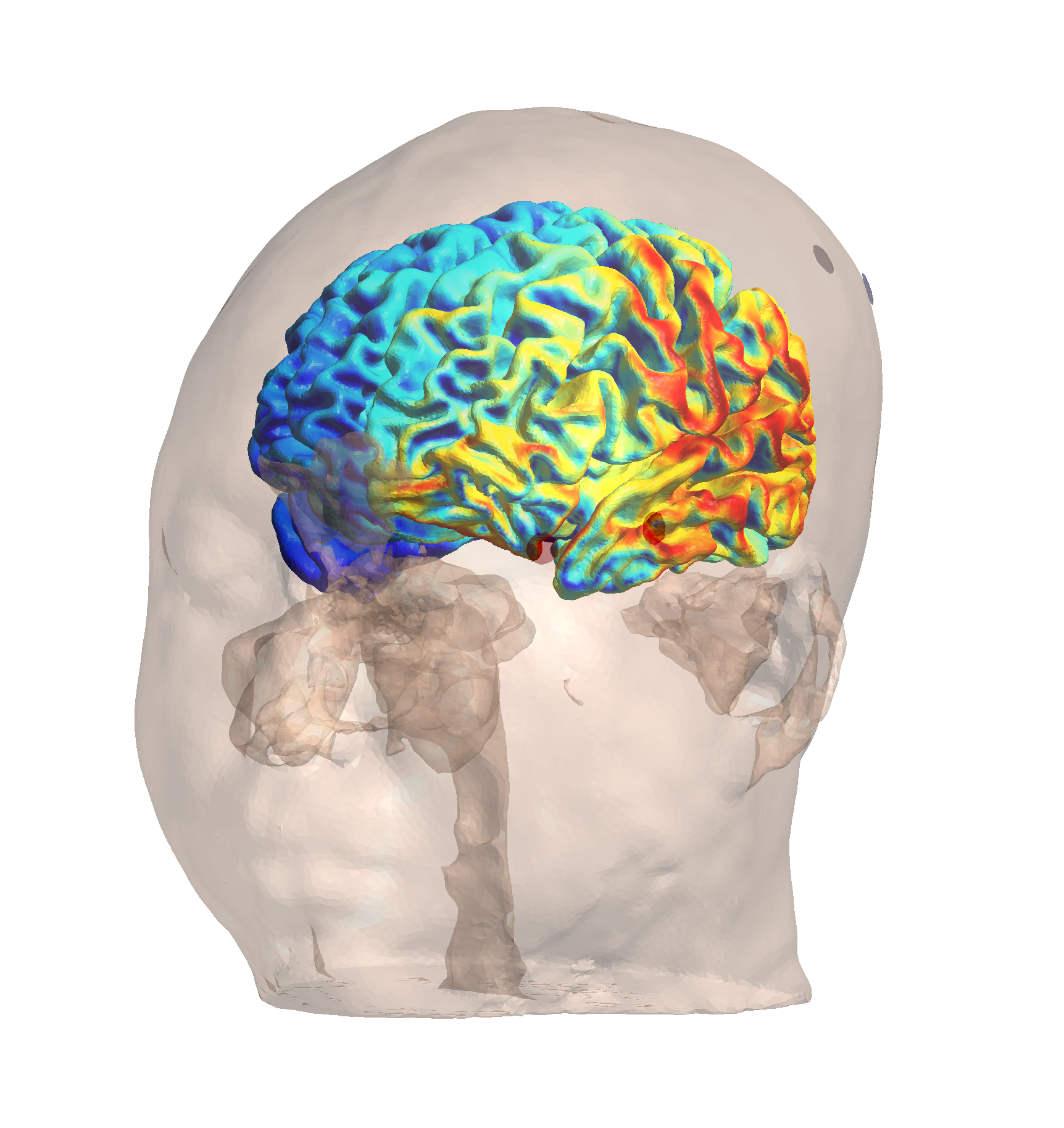The field component tangential to the cortical surface.

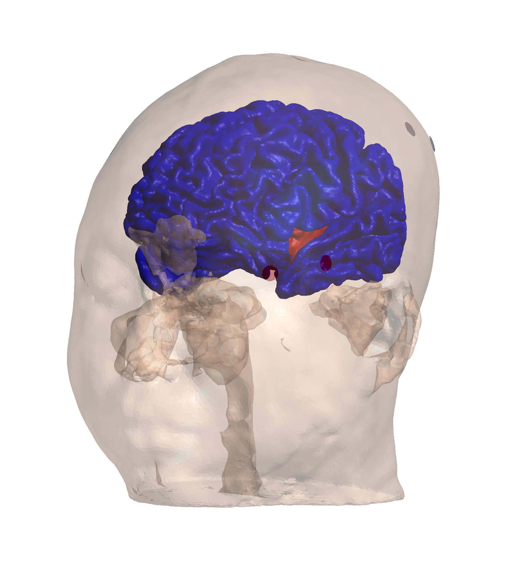The tangential component restricted to the target ROI.

Simulating a candidate on a cap

In Simulator, use the placement selector to keep Optimised (XYZ) or snap the selected candidate to a subject cap. Snapping assigns distinct cap sites to this candidate, preserves its currents and electrode settings, and replaces the optimized poses with the cap placement. Switching back restores the recorded XYZ and orientations. The preview highlights the selected cap sites, with hollow original positions and dashed displacement links. Distances are straight-line millimetres, not distances along the scalp. Optimization metrics describe the original candidate; evaluate the snapped montage with a new simulation.