Simulator
The Simulator computes the full FEM temporal interference field. It sits between the optimizers and the analyzer: take a montage from the montage list or from a flex-search or ex-search result, or placed by hand and simulate it here. Then, quantify the resulting field with the Analyzer. It can be invoked programmatically via run_simulation() or through a JSON config entrypoint.
In the application
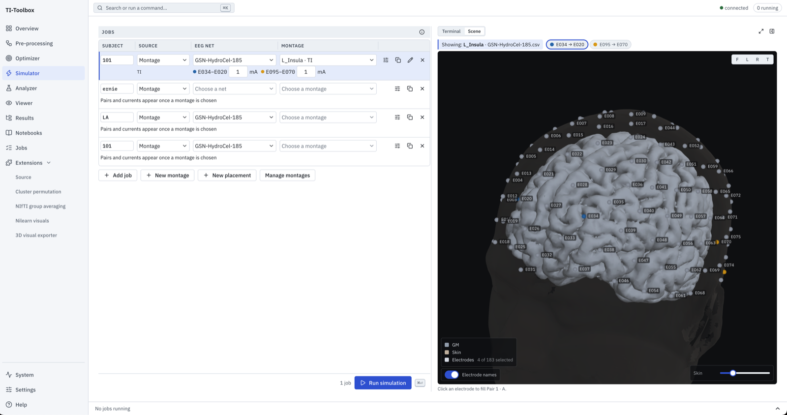 The Simulator (⌘3). One row is one job; the pane beside it draws that montage on the selected subject.
- Subject Selection: Choose from available pre-processed subjects; multiple subjects can be queued for batch processing
- Montage Source: Per-job drop-down —
Montage,Flex-Search, orFreehand(see Montage Sources) - Simulation Mode: Unipolar/multipolar with per-channel current inputs
- EEG Net: Dropdown selection of available electrode configurations
- Conductivity Model: Four anisotropy types (
scalar,vn,dir,mc) with configurable bounds (see Conductivity and Anisotropy) - Output Fields: Checkboxes for
TI_max(default),TI_avg,hf_peakandhf_sar; at least one must be selected - Real-time Logging: Simulation progress and status updates
Montage Sources
The simulator supports three primary montage source types:
1. Montage List
Pre-defined electrode configurations organized by EEG net and stimulation mode:
- Unipolar Montages: Standard TI — 4 electrodes forming 2 channels
- Multipolar Montages: mTI — 8 electrodes forming 4 channels, for higher focality
- EEG Net Compatibility: Automatically filtered based on selected electrode configuration
- Management: Add, remove, and refresh montage collections
2. Flex Mode
Automatic integration with the flex-search optimizer.
- Optimize: Start by running the optimizer based on your needs
- Simulate: Move to the simulator and use the automatic montage available from the flex-search
- Run Identity: Flex-search-derived simulations keep their unique run IDs on disk, while the UI shows concise display names and hover metadata so repeated simulations are easier to distinguish without long folder labels.
3. Free-Hand
Mode that allows exploration of untraditional montages
- Flexible Positioning: Manual electrode placement for specialized protocols
- New placement: Use the Simulator’s built-in placement editor to place electrodes on the subject’s scalp
Available EEG Nets
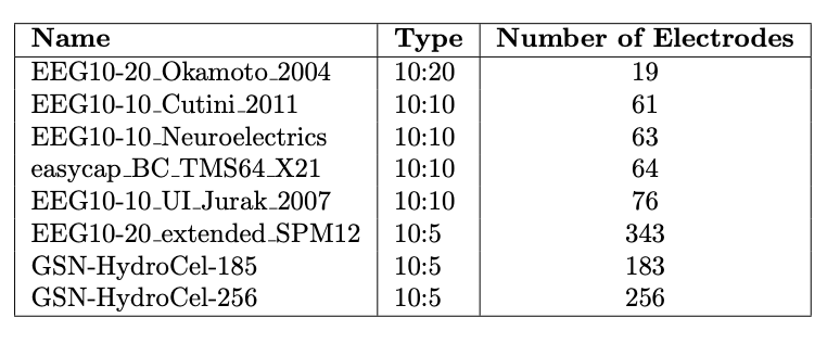
The TI-Toolbox automatically co-registers these EEG electrode nets to head models during preprocessing, so no manual registration step is needed — the same pre-aligned nets serve simulation, flex-search electrode mapping, and leadfield generation. The GUI scans eeg_positions/ directories for available configurations, refreshes montage lists when the selected net changes, and displays only montages compatible with that net.
Simulation Modes
Unipolar Mode
- Configuration: Two electrode pairs (four electrodes), forming two channels whose slightly different frequencies produce the TI envelope
- Current Settings: One current magnitude per channel; each channel has an active and return electrode
- Applications: Standard two-channel temporal interference stimulation
- Montage Compatibility: Works with unipolar montage collections
Multipolar Mode (mTI)
Standard TI uses 4 electrodes forming 2 channels (a channel = one electrode pair driven by one current source); the two channels share one carrier — e.g. 2.000 and 2.010 kHz around a 2 kHz carrier — and their beat is the TI envelope. Multipolar temporal interference (mTI) doubles this: 8 electrodes form 4 channels, and each two channels share a carrier (e.g. channels 1 & 2 near 2 kHz, channels 3 & 4 near 4 kHz). Each carrier produces its own beat, and the beats — all at the same difference frequency and phase-aligned — combine into one modulation envelope (Botzanowski et al. 2025, who drove up to 4 carriers / 8 channels / 16 electrodes; their Supplementary Fig. 1 shows that envelopes offset in phase weaken the aggregate and cancel it entirely at 180°).
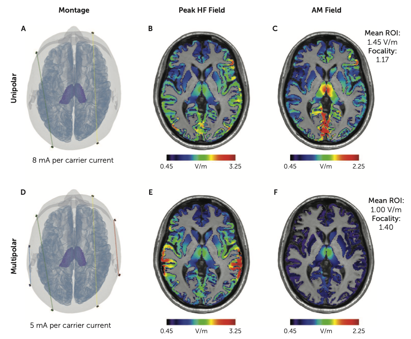 Unipolar (top, A–C) vs. multipolar (bottom, D–F) TI targeting the same deep ROI. Left: electrode montage — two channels at 8 mA each vs. four channels at 5 mA each. Middle: peak high-frequency field. Right: the amplitude-modulated (AM) envelope field that actually drives neurons. The multipolar montage trades some ROI intensity (mean 1.00 vs. 1.45 V/m) for a more focal envelope (focality 1.40 vs. 1.17) and a lower per-channel current. Adapted from Albantakis & Tononi 2026, American Journal of Psychiatry.
- Configuration: Any even number of channels, 4 or more — i.e. 8+ electrodes (capped at 26 channels, labelled A–Z)
- Current Settings: One current input per channel (see Simulator Behavior for mTI below)
- Applications: Distributed stimulation, field steering, and complex targeting
- Montage Compatibility: Works with multipolar montage collections
For the envelope field math behind these quantities see Envelope Math and Critical Values on the Analyzer page.
How the Toolbox Detects mTI
TI vs. mTI is not a setting – it is inferred purely from how many channels (electrode pairs, in the code’s wording) a montage has. Montage.simulation_mode (tit/sim/config.py) does this:
- 2 channels ->
SimulationMode.TI - 4 or more channels ->
SimulationMode.MTI - 0, 1, or 3 channels -> raises
ValueError("Invalid number of electrode pairs: {n}. Expected 2 (TI) or 4+ (mTI).")
There is no odd-channel-count mTI: an mTI montage must have an even number of channels (every carrier needs two), and mTISimulation additionally caps it at 26 channels (see Simulator Behavior for mTI below).
Montages are persisted in montage_list.json under separate keys per EEG net:
data["nets"][eeg_net]["multi_polar_montages"][name] = [[e1,e2],[e3,e4],[e5,e6],[e7,e8]]
data["nets"][eeg_net]["uni_polar_montages"][name]   = [[e1,e2],[e3,e4]]
upsert_montage(..., mode="M") writes to multi_polar_montages; mode="U" writes to uni_polar_montages. When a montage is loaded by name, load_montages resolves it as multi.get(name) or uni[name] – if the same name exists in both dictionaries, the multi-polar entry wins.
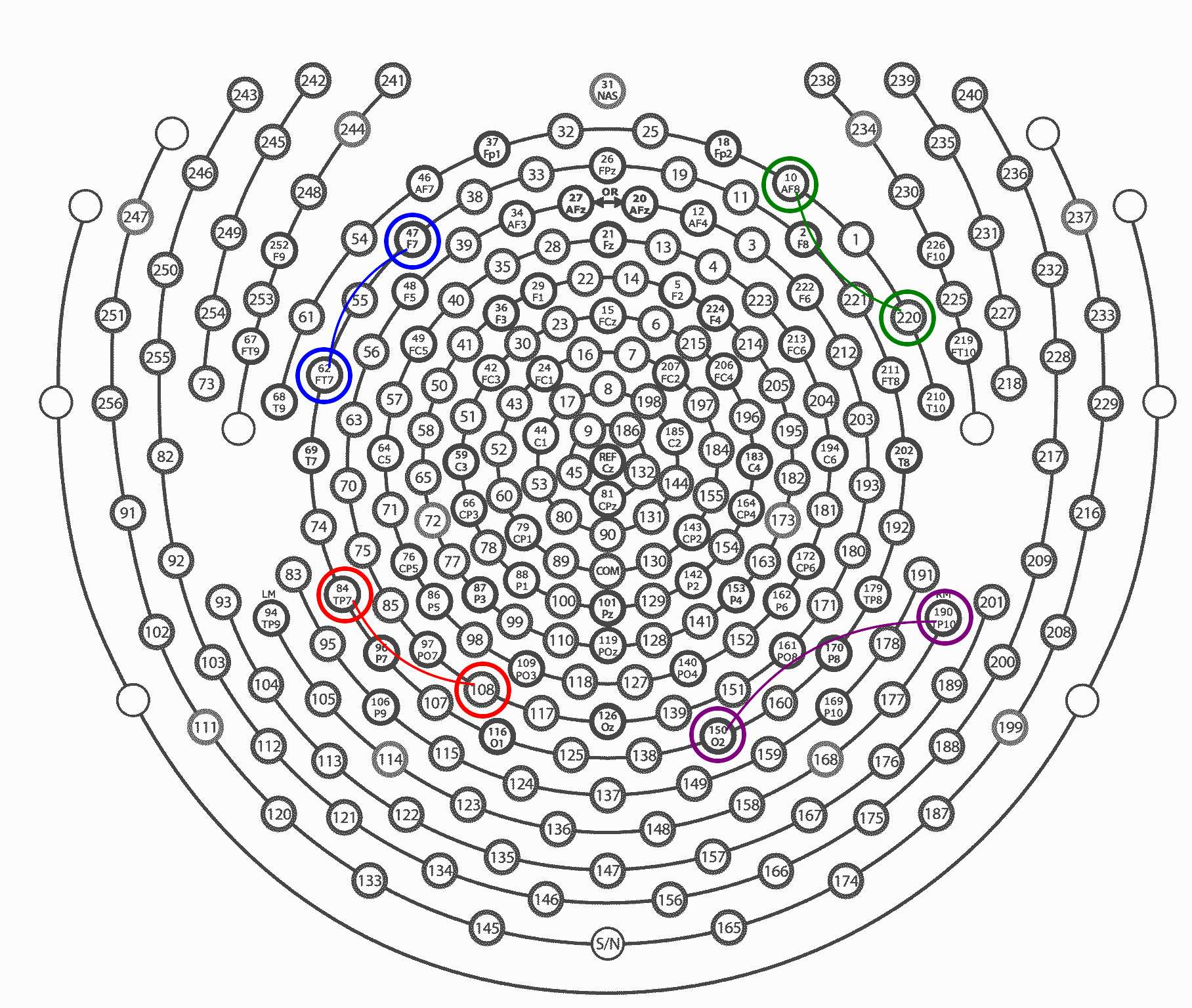 A multipolar montage: 8 electrodes forming 4 channels on 2 carriers.
Channels and Carriers
The assignment is always positional: each two consecutive electrodes in the montage compose a channel, and each two consecutive channels compose a carrier. For an 8-electrode montage that means channels A & B share the first carrier and channels C & D the second — there is no wiring choice to make.
The kHz-exposure safety metrics hf_peak/hf_sar include every channel field under the shipped positional wiring (one field per carrier). Their math lives under Safety Metrics on the Analyzer page.
Simulator Behavior for mTI
mTISimulation (tit/sim/mTI.py) builds one SimNIBS TDCS list per channel, each driven at config.intensities[i] mA (converted to A). SimulationConfig.intensities defaults to [1.0, 1.0]; for mTI, validation requires len(config.intensities) >= montage.num_pairs – one current value per channel, not two. The GUI’s job-card current placeholder switches from 1.0,1.0 to 1.0,1.0,1.0,1.0 when the montage mode is multipolar.
On disk, the mTI mesh spells the modulation-depth field mTI_max – the same quantity TI_max names on a standard TI mesh, just a different on-disk name for the multipolar case.
TI_normal is computed for mTI too. Standard TI derives it from SimNIBS’s 2-field TI.get_dirTI; mTI evaluates the same \(K\)-carrier envelope at a fixed direction — the cortical surface normal — via tit.calc.get_TI_dir over all N channel overlays, and writes it as {montage}_mTI_normal.msh in mTI/mesh/.
fsaverage projection covers mTI. Enable Map fields to fsaverage in each job’s settings to project its fields after simulation. New UI jobs start with mapping off; new rows inherit the last configured job settings. The Python SimulationConfig.map_to_fsavg default remains True for existing scripts. Projection runs for both modes; for mTI it reads the modulation depth from the mTI central surface (field mTI_max) and derives hf_peak/hf_sar from all N channel volume meshes.
mTI supports an arbitrary even number of channels, capped at 26 (A-Z channel labelling); more than 26 channels raises ValueError. Post-processing:
- Loads and crops all N high-frequency meshes to brain tissue (
BRAIN_TISSUE_TAG_RANGES = ((1, 100), (1001, 1100))). - Computes an intermediate per-carrier TI vector field for each consecutive channel pair (
{montage}_TI_AB.msh,{montage}_TI_CD.msh, …) via the plain single-carrierget_TI_vectors– these are saved for inspection only and are not recombined into the final result (a recursive TI-of-TI recombination is not a valid envelope). - Computes the final envelope over all N channel fields jointly via
get_TI_vectors(e_fields), written asmTI_max; optionallyTI_avg,hf_peak,hf_sarperoutput_fields. - Extracts GM/WM crops (
grey_{montage}_mTI.msh,white_{montage}_mTI.msh), generates a central cortical surface viamsh2cortex, and converts meshes to NIfTI.
Per-channel high-frequency meshes are renamed TDCS_1..N -> TDCS_A..Z when moved into high_Frequency/mesh/, matching the A-Z channel labelling used everywhere else in the mTI output.
References: Albantakis, L. & Tononi, G. (2026). Precision neuromodulation in psychiatry: focus on temporal interference stimulation. American Journal of Psychiatry. doi:10.1176/appi.ajp.20250873. Botzanowski, B. et al. (2025). Focal control of non-invasive deep brain stimulation using multipolar temporal interference. Bioelectronic Medicine 11(1):7.
Output Fields
SimulationConfig.output_fields gates which volume-mesh fields are computed and written – it defaults to ["TI_max"] only. TI_avg and the safety fields (hf_peak, hf_sar) must be opted into; the four selectable names are exactly ("TI_max", "TI_avg", "hf_peak", "hf_sar") (const.SELECTABLE_OUTPUT_FIELDS). The gating skips the computation, not just the write – unrequested fields are never evaluated. In the GUI (shared by TI and mTI), output fields are checkboxes with only TI_max pre-checked; submitting with none checked is rejected with “Select at least one output field.”
What each field means — the beat-envelope modulation depth, the direction-averaged envelope, and the carrier-exposure safety metrics — is documented once, under Quantities of Interest on the Analyzer page.
Conductivity and Anisotropy
The conductivity string field on SimulationConfig (or the GUI dropdown) selects one of four tissue conductivity models:
| Type | Code | Description | Requirements |
|---|---|---|---|
| Scalar | scalar |
Isotropic, piecewise-constant (default) | None — used when no DTI data is available |
| Volume Normalized | vn |
Normalized tensors scaled by tissue conductivity | DTI tensor |
| Direct | dir |
Direct linear rescaling of diffusion tensor eigenvalues | DTI tensor |
| Mean Conductivity | mc |
Isotropic but spatially varying, from tensor volumes | DTI tensor |
The anisotropic models account for fiber orientation, giving more realistic modeling of white matter tracts. Two additional SimulationConfig parameters bound them: aniso_maxratio (default: 10.0, maximum ratio between eigenvalues) and aniso_maxcond (default: 2.0, maximum conductivity value).
DTI Data Preparation
The TI-Toolbox provides integrated DTI processing: QSIPrep preprocesses the diffusion data and the DTI step fits the tensor with DIPY and writes it in the format SimNIBS reads. For anisotropic simulation, the following file must exist in the m2m directory:
derivatives/SimNIBS/sub-{id}/m2m_{id}/
└── DTI_coregT1_tensor.nii.gz    # 4D tensor (X, Y, Z, 6)
For complete DTI processing instructions, see the Diffusion Processing documentation; for the underlying theory, see the SimNIBS dwi2cond documentation.
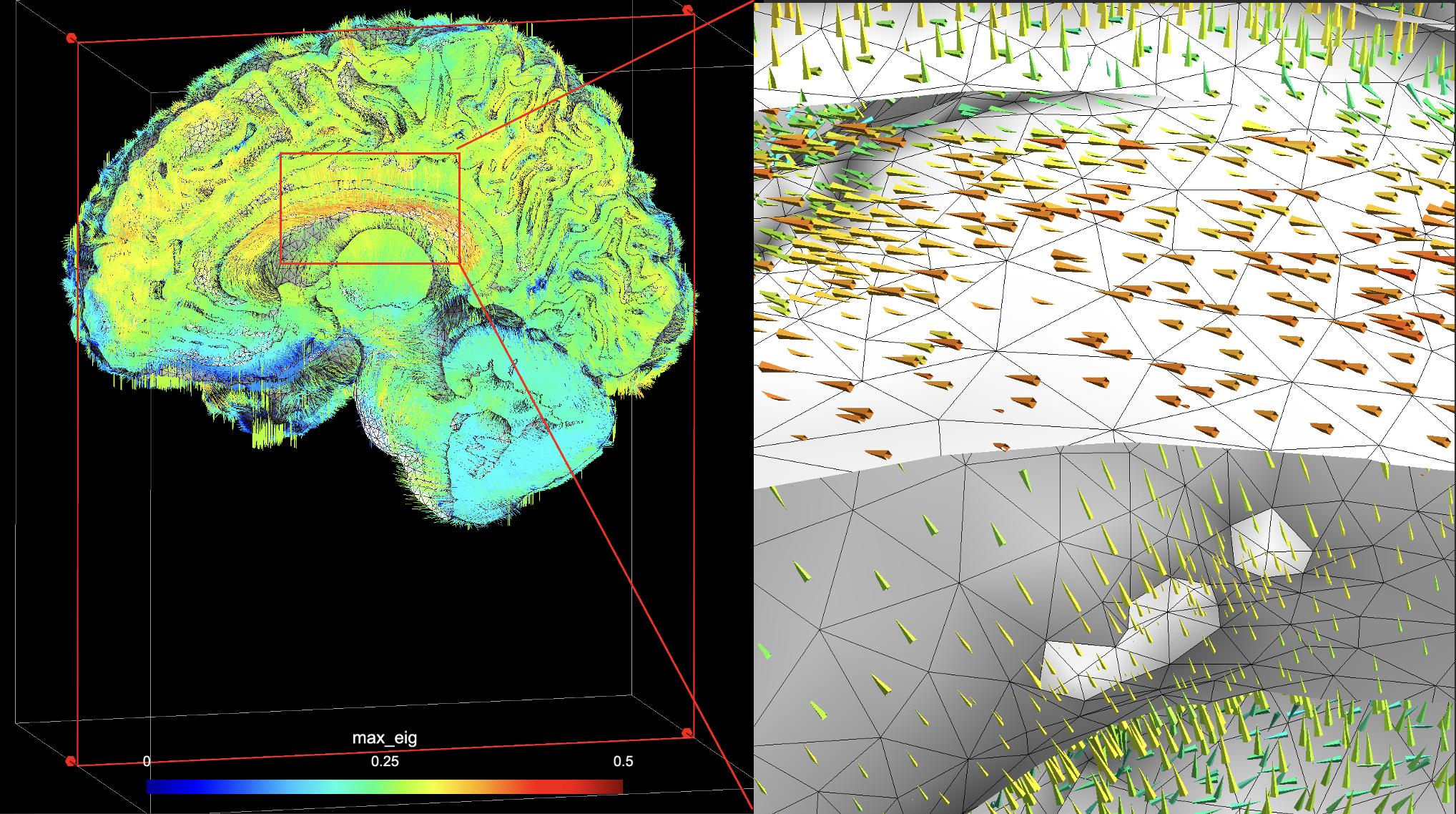
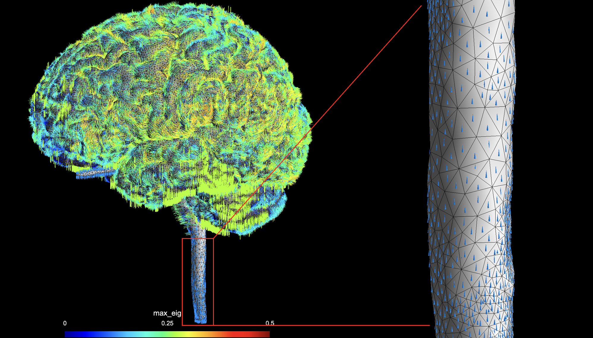
White and gray matter with overlaid eigen vectors that scale conductivity in anisotropic simulations. Top: Corpus callosum region showing organized fiber directions. Bottom: Spinal cord region with longitudinal fiber orientation.
Output Layout and CLI
derivatives/SimNIBS/sub-{ID}/Simulations/{montage}/
├── documentation/config.json            # provenance snapshot used by the report
├── high_Frequency/{mesh,niftis,analysis} # per-channel SimNIBS outputs
├── TI/                                   # standard TI (2 channels)
│   ├── mesh/{montage}_TI.msh, grey_*.msh, white_*.msh
│   ├── niftis/{montage}_TI_subject_TI_max.nii.gz (+ _MNI_ when MNI export is on)
│   ├── montage_imgs/{montage}_highlighted_visualization.png
│   └── surface_overlays/
└── mTI/                                  # multipolar TI (4+ channels)
    ├── mesh/{montage}_mTI.msh            # mTI_max / TI_avg / hf_peak / hf_sar (selected)
    ├── mesh/grey_{montage}_mTI.msh, white_{montage}_mTI.msh
    ├── mesh/surfaces/                    # central cortical surface (msh2cortex)
    ├── niftis/                           # mesh -> NIfTI conversion
    └── montage_imgs/                     # combined_montage_visualization.png
NIfTI exports are written in subject space by default. Enable Generate MNI NIfTI outputs beside the fsaverage option in job settings to also export MNI fields and the MNI anatomical reference — ROI inputs elsewhere in the toolbox accept either space, with automatic transformation between them.
The GUI writes a JSON config and runs simnibs_python -m tit.sim config.json; the same command works from a shell (see Scripting for the SimulationConfig fields).
Report generation
Every simulated montage writes a simulation report, from the app, run_simulation() or a JSON config alike: the grey-matter envelope and where its maximum is, the montage on the EEG cap with its dose, and the envelope in three planes. Rebuild one without re-simulating with simnibs_python -m tit.reporting.generators.simulation <project> <subject> <simulation>. See Reports.