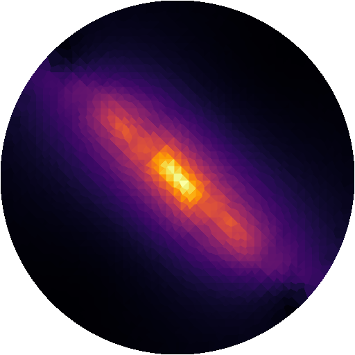
Ex-Search TI Optimization Pipeline

Ex-Search is the toolbox’s exhaustive montage optimizer: it evaluates every electrode combination (× every current split) you allow, on a precomputed leadfield, and ranks the results. Unlike Flex-Search, which freely positions electrodes on the scalp with a stochastic optimizer, ex-search is restricted to the electrodes of an EEG net — but within that space it is guaranteed to find the global optimum, and each candidate costs milliseconds.

Prerequisites: Leadfield and EEG Net

Every ex-search runs against a leadfield matrix for one subject and one EEG net. The GUI scans for existing leadfields, validates the HDF5, and can create new ones for any supported net (leadfields are 2–20 GB depending on the number of electrodes). EEG nets are automatically co-registered during pre-processing:

[INFO] Scanning available EEG nets for subject 101...
  1. BioSemi-64-10-10.csv
  2. BioSemi-128-A1.csv
  3. BioSemi-256-A1.csv
  4. EEG10-10_Cutini_2011.csv
  5. EEG10-10_UI_Jurak_2007.csv
  6. EEG10-20_Okamoto_2004.csv
  7. GSN-HydroCel-128.csv
  8. GSN-HydroCel-185.csv        # Default selection
  9. GSN-HydroCel-256.csv
 10. easycap_BC_TMS64_X21.csv

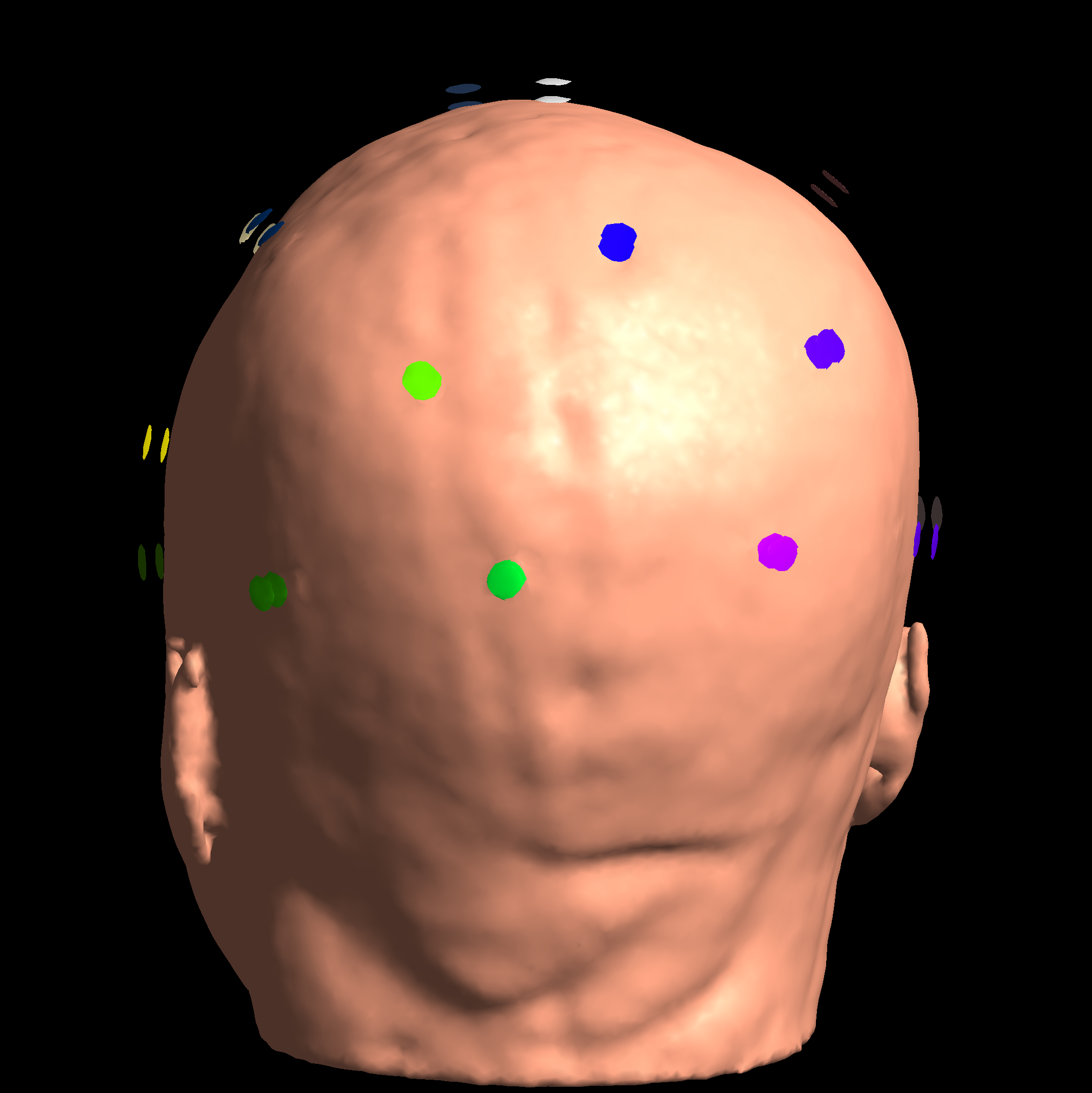EEG 10-20 Okamoto 2004 electrode configuration - widely used standard with 32 electrodes

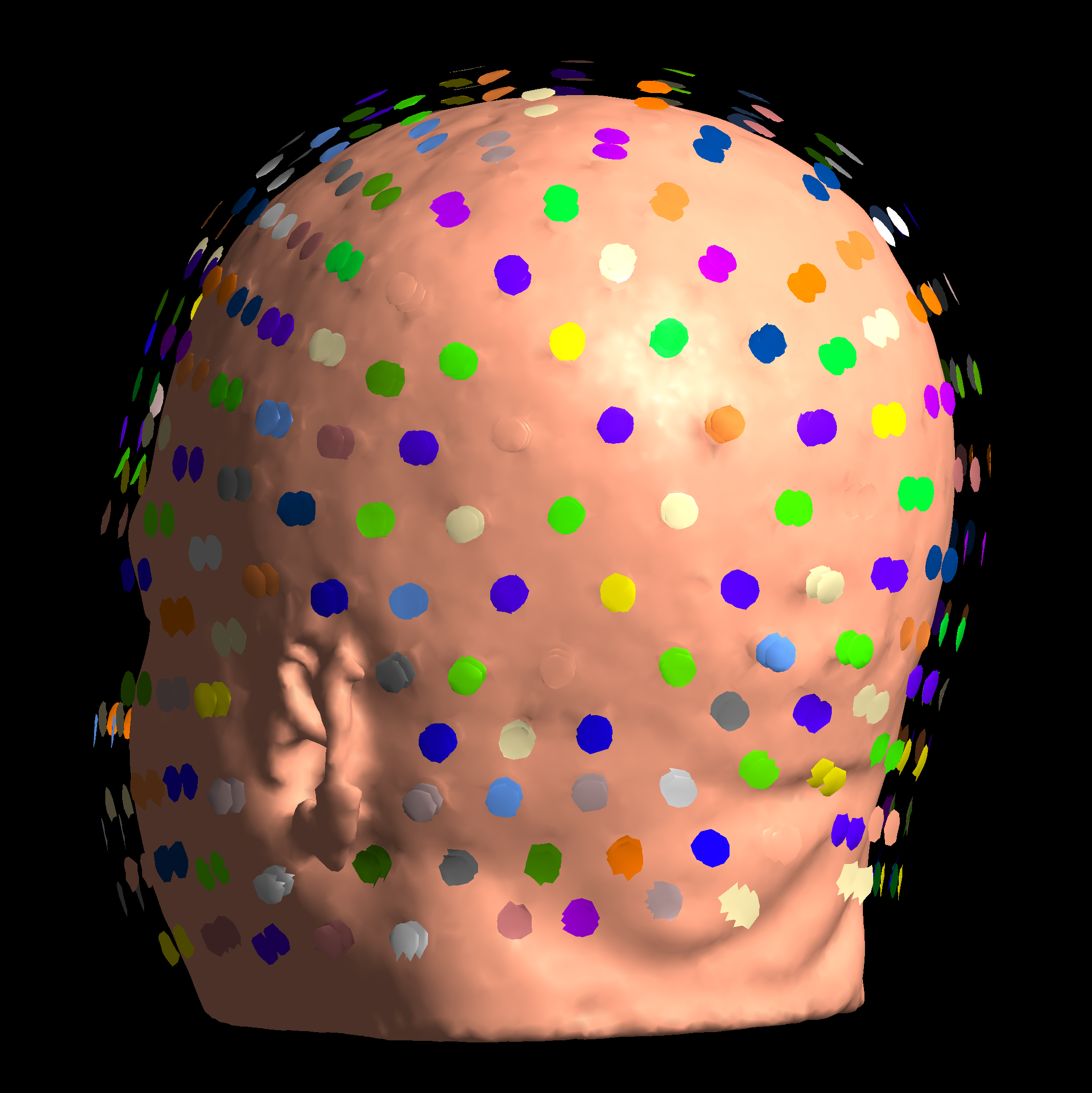GSN-HydroCel 256 electrode configuration - high-density net for precise targeting

Leadfields are generated with tissues=[1, 2] (white + grey matter).

User Interface

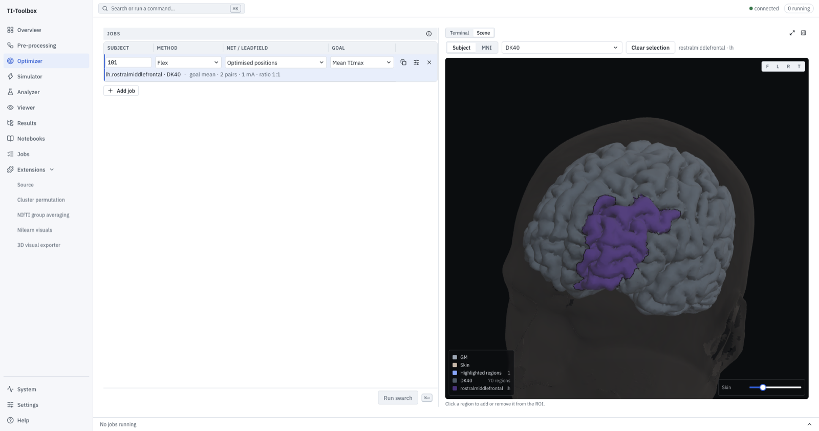Ex-search is the Ex method on the Optimizer page (⌘2), not a page of its own; the row shown uses Flex.

The interface provides controls for:

• Subject Selection: Choose from available subjects with automatic leadfield scanning
• Leadfield Management: View existing leadfields, create new ones, and show electrode configurations
• ROI Selection: see Defining the Target
• Electrode Setup: Configure E1+, E1-, E2+, E2- with support for both GSN and 10-20 formats
• Execution Control: Run optimization with real-time progress tracking

Defining the Target (ROI)

The Target section offers three choices:

• Saved uses saved spherical ROI CSVs, a radius, and Subject/MNI coordinates. “Combine selected ROIs into one target” unions the selected centers for a single Ex search.
• Subcortical selects regions from a volumetric atlas.
• NIfTI mask imports a local .nii or .nii.gz file into the project. Positive voxels define the target. Subject-space masks are used directly; MNI masks use the subject’s SimNIBS registration in m2m_<subject>/toMNI, with nearest-neighbor resampling. The conformation affine alone is not an MNI registration.

Electrodes is a separate section: choose four electrodes (TI) or eight (mTI), then configure the search space.

Under the hood, ROI resolution OR-folds a mixed list of CSV centers, whole NIfTI/MGZ masks (voxel value > 0), and (path, label) atlas-region selections (voxel value == label) into a single region.

Defining the Search Space

Bucket Mode

electrodes are pre-assigned to specific channels:

• E1+: Electrodes for positive channel 1
• E1-: Electrodes for negative channel 1
• E2+: Electrodes for positive channel 2
• E2-: Electrodes for negative channel 2

Combinations: \(N_1 \times N_2 \times N_3 \times N_4\), where \(N_i\) is the number of electrodes in bucket \(i\).

Pool Mode

All electrodes are pooled together and can be assigned to any channel position, with the constraint that each electrode is used only once per montage.

Combinations: \(\binom{N}{4} \times 4!\), where \(N\) is the total number of electrodes — every 4-electrode subset in every channel assignment.

Trade-off: Larger search space and longer compute time but with absolute certainty to find optimal solution with given electrode space.

Symmetric (Bilateral) Constraint

Bucketed searches can be restricted to left/right-mirrored montages with symmetric_bucket: true. The mirror map is read from the EEG-position CSV (symmetry_eeg_csv; inferred from the leadfield name {subject}_leadfield_{net}.hdf5 when omitted). Two pairings:

• symmetry_pairing: "within_pairs" — each channel is bilateral: E1- must be the mirror of E1+ and E2- of E2+ (e.g. F7_F8 <> TP7_TP8). Write left candidates in the + buckets and their mirrors in the - buckets.
• symmetry_pairing: "cross_pairs" — channel 2 is the mirror of channel 1: E2+ = mirror(E1+), E2- = mirror(E1-) (e.g. F5_TP7 <> F6_TP8).

Current ratios

On top of the electrode combinations, the search systematically tests current splits between the two channels, respecting an optional per-channel limit:

Example (non-default; defaults are total_current=2.0 mA, current_step=0.5 mA, no channel_limit):
For total_current=2.0mA, step=0.2mA, limit=1.6mA:
  (1.6, 0.4), (1.4, 0.6), (1.2, 0.8), (1.0, 1.0),
  (0.8, 1.2), (0.6, 1.4), (0.4, 1.6)

The editor shows montage counts and total iterations separately. For fixed balanced currents, set the channel limit to half the total current (with a step no larger than that half); there is one split and iterations equal montages.

Total evaluations = electrode combinations × current ratios. Each montage’s two unit-current channel fields are computed once and rescaled per split — the FEM is linear, so a split costs almost nothing extra.

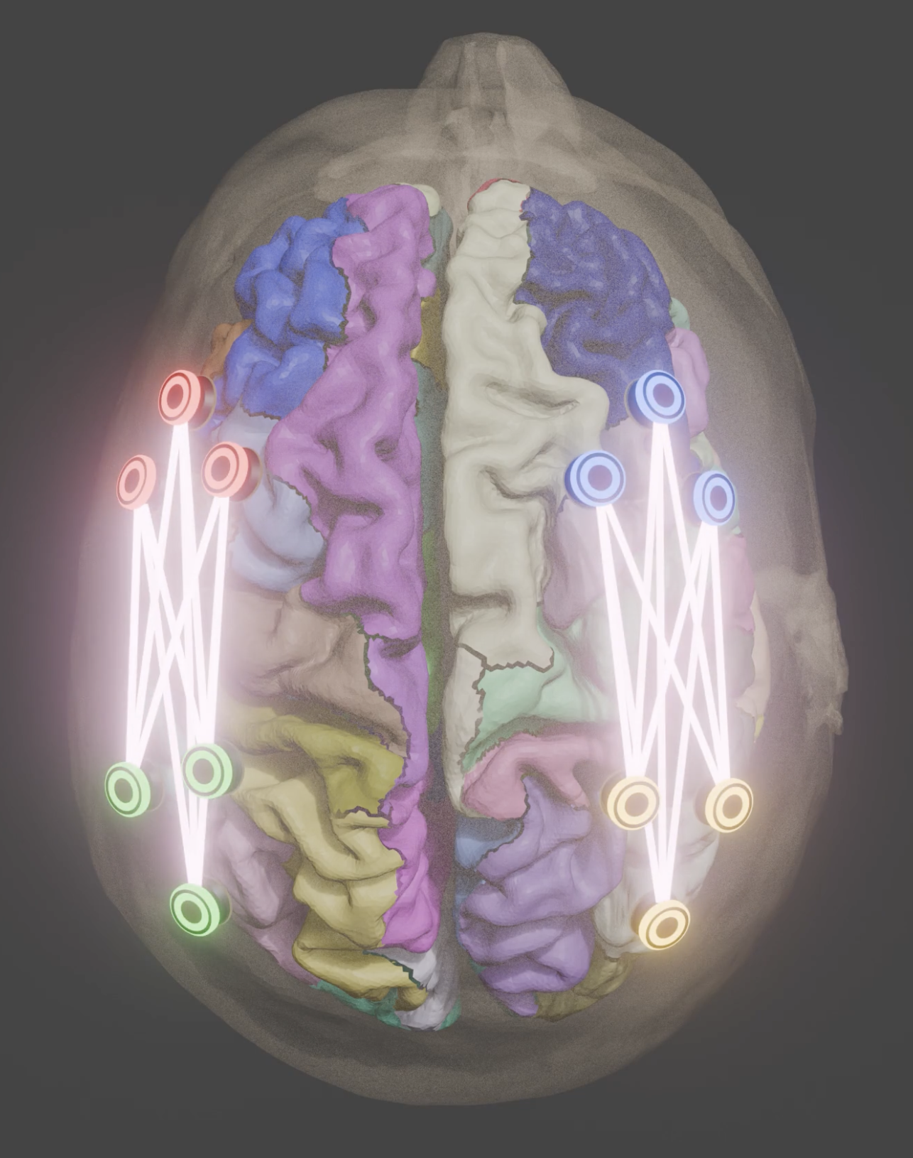Example candidate electrode combinations. The final search size is determined by the selected pools or buckets, symmetry constraints, and current splits.

Running a Search

The GUI writes a JSON config and runs the module; the same works from a shell:

simnibs_python -m tit.opt.ex config.json

All computation is in-memory (no intermediate mesh files), with constant memory footprint regardless of combination count, real-time progress and ETA tracking, and graceful interruption: SIGINT/SIGTERM sets a stop flag that breaks after the current candidate, and partial results are still written. Candidates are spread over worker processes (n_jobs, default the CPU limit from Settings → Project → Execution, 70 % of the cores; larger values are capped at it). Run time ranges from minutes to hours depending on leadfield size and combination count.

Outputs

Metrics

Every evaluated candidate is scored on the closed-form two-channel TI envelope (TI_max; the math lives on the Analyzer page), evaluated on ROI grey matter only:

Key	Meaning
TImax_ROI	Max over ROI elements
TImean_ROI	Volume-weighted mean over ROI elements
TImean_GM	Volume-weighted mean over GM elements (SimNIBS tag 2)
Focality	TImean_ROI / TImean_GM
Composite_Index	TImean_ROI × Focality
n_elements	ROI element count

Focality here has the same definition as the analyzer’s roi_focality, so search results and post-hoc analyses are directly comparable.

Files

Each run writes to derivatives/SimNIBS/sub-{id}/ex-search/{run_name}/:

• run_config.json — provenance snapshot of the search configuration.
• final_output.csv — one row per evaluation. The Montage column carries the current split as a suffix (e.g. F7_CP5 <> AF7_P3_I1-1.0mA_I2-1.0mA); currents are written with one decimal, so a 0.25 mA step appears as 0.2/0.8/1.2/1.8 in the CSV.
• Five PNG figures: montage_distributions.png (histograms of TImax, TImean, focality), intensity_vs_focality_scatter.png, and three EEG-map figures — electrode_score_heatmap.png (electrode participation across the top-50 montages: colour = summed Composite Index, size = frequency), montage_strength_map.png and montage_focality_map.png (the top-150 montages drawn as arcs on the cap, coloured by TImean_ROI / Focality, best montage highlighted). The maps need the net’s EEG-position CSV (resolved like symmetry_eeg_csv) and are skipped with a log line otherwise; regenerate them for an existing run with simnibs_python -m tit.opt.ex.results <run_dir> [--eeg-csv CSV].

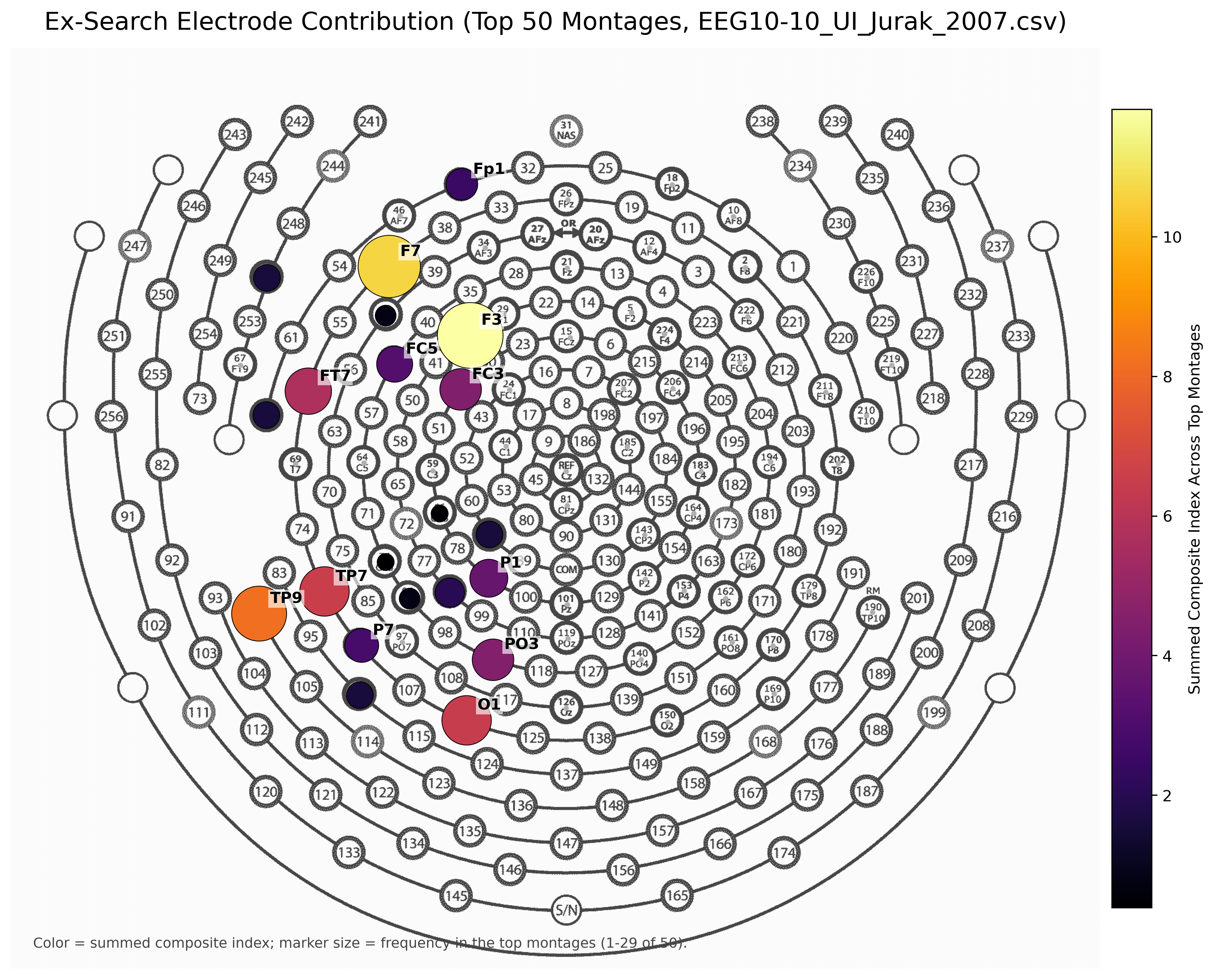
electrode_score_heatmap.png — which electrodes recur in the best montages (16,807-evaluation run)

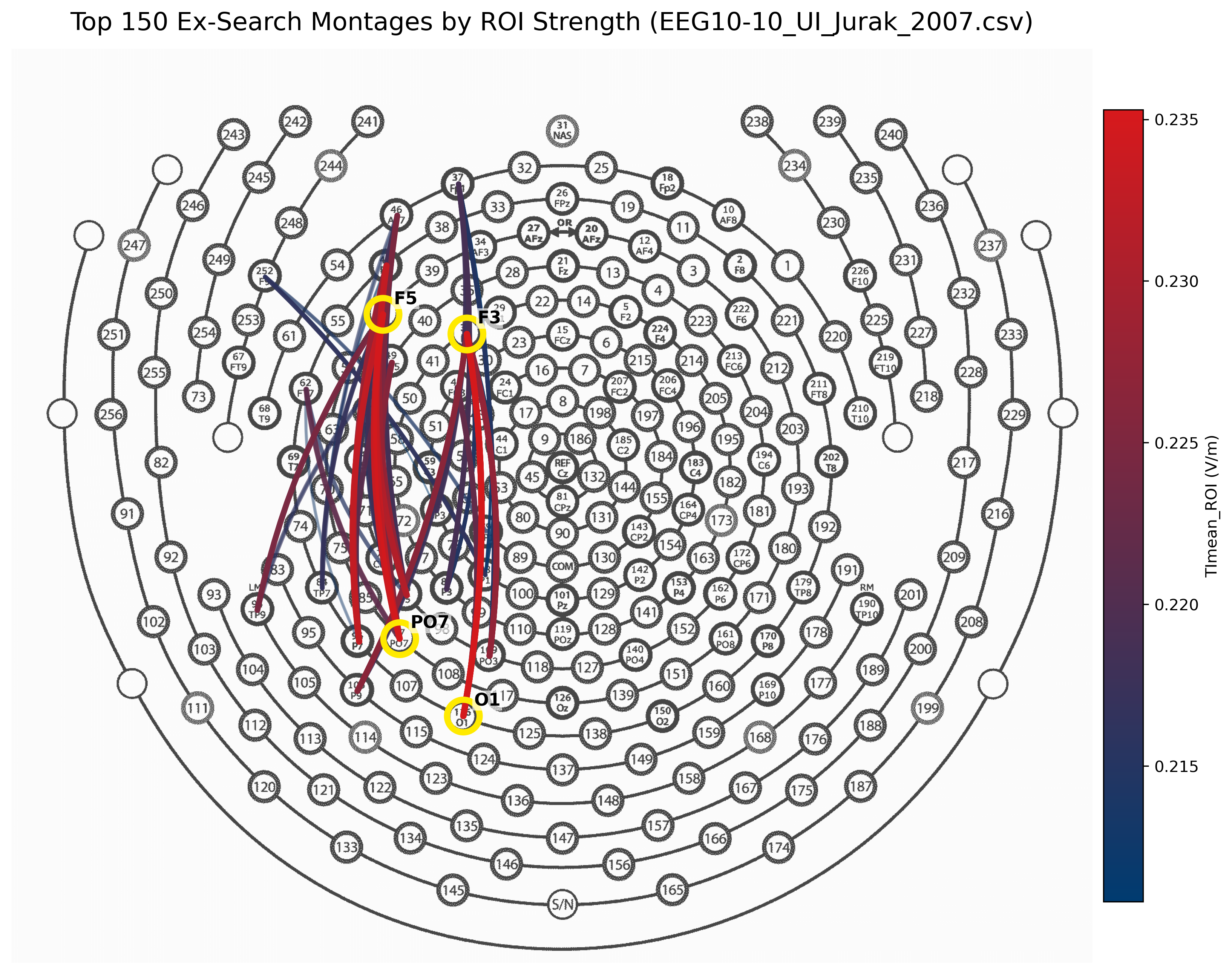
montage_strength_map.png — top-150 montages by ROI strength

Example Results

Top 5 of 16,807 evaluations by Composite_Index (sub-ernie, EEG10-10 Jurak leadfield, 5 mm spherical ROI at MNI (−38, 5, 0), TI-Toolbox v2.4.0). Bucket search with 7 candidate electrodes per position (7⁴ = 2,401 electrode combinations) × 7 current splits (2 mA total, 0.25 mA step) — 13.6 min on 12 cores (0.05 s each):

Montage	Current_Ch1_mA	Current_Ch2_mA	TImax_ROI	TImean_ROI	TImean_GM	Focality	Composite_Index
F7_TP9 <> F3_P1	1.0	1.0	0.3561	0.2066	0.0959	2.1553	0.4454
F7_TP9 <> F3_PO3	1.0	1.0	0.3766	0.2103	0.1024	2.0545	0.4320
FT7_TP9 <> FC3_P1	1.0	1.0	0.3637	0.1819	0.0771	2.3585	0.4291
F7_TP7 <> F3_P3	1.0	1.0	0.3451	0.2109	0.1050	2.0091	0.4237
F7_TP9 <> F3_O1	1.0	1.0	0.3766	0.2103	0.1047	2.0092	0.4225

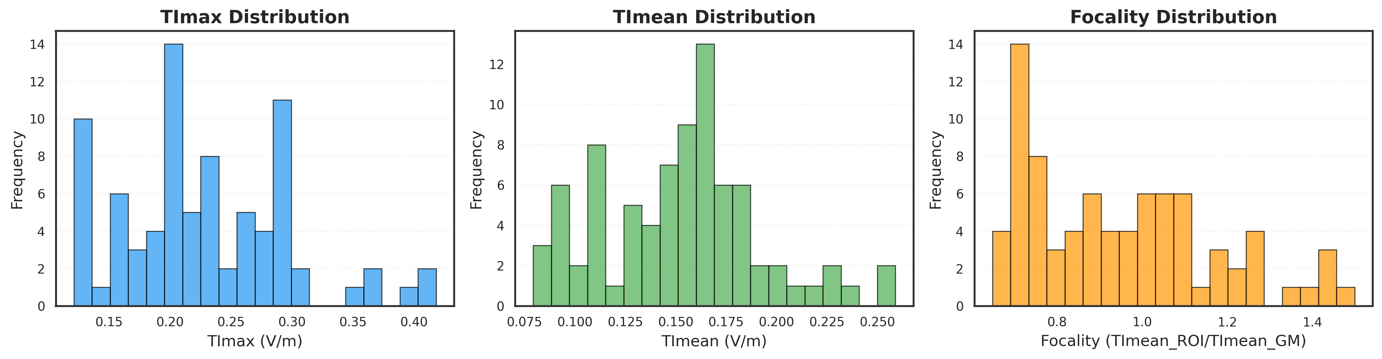
montage_distributions.png from the same run: TImax, TImean and focality across all 16,807 evaluations.

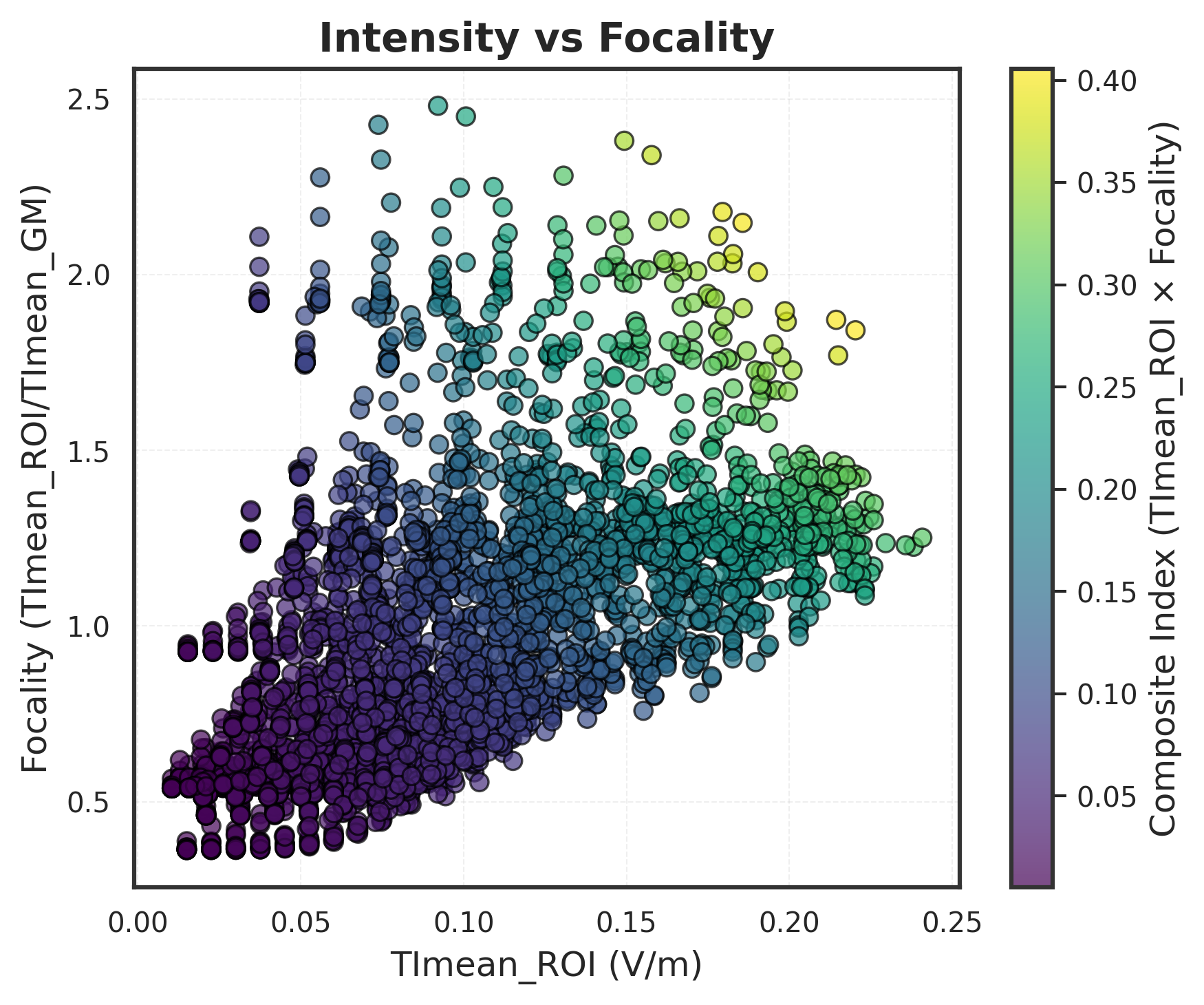
intensity_vs_focality_scatter.png: every evaluation plotted as ROI mean intensity against focality, coloured by Composite_Index. With ~17k candidates the Pareto front emerges along the upper-right edge — no montage improves intensity without giving up focality beyond it. Equal 1.0/1.0 mA splits populate the high-intensity end; strongly unequal splits (0.2/1.8) collapse to the low-intensity cluster on the left.

Symmetric example

within_pairs, 7 bilateral candidates per channel × 7 current splits = 343 evaluations on sub-ernie (18 s):

Montage	Ch1 mA	Ch2 mA	TImax_ROI	TImean_ROI	TImean_GM	Focality	Composite_Index
FT7_FT8 <> TP7_TP8	0.8	1.2	0.4371	0.2290	0.1150	1.9909	0.4560
FT7_FT8 <> CP5_CP6	0.8	1.2	0.4404	0.2285	0.1145	1.9949	0.4558
F7_F8 <> TP7_TP8	0.8	1.2	0.3964	0.2021	0.0938	2.1540	0.4353

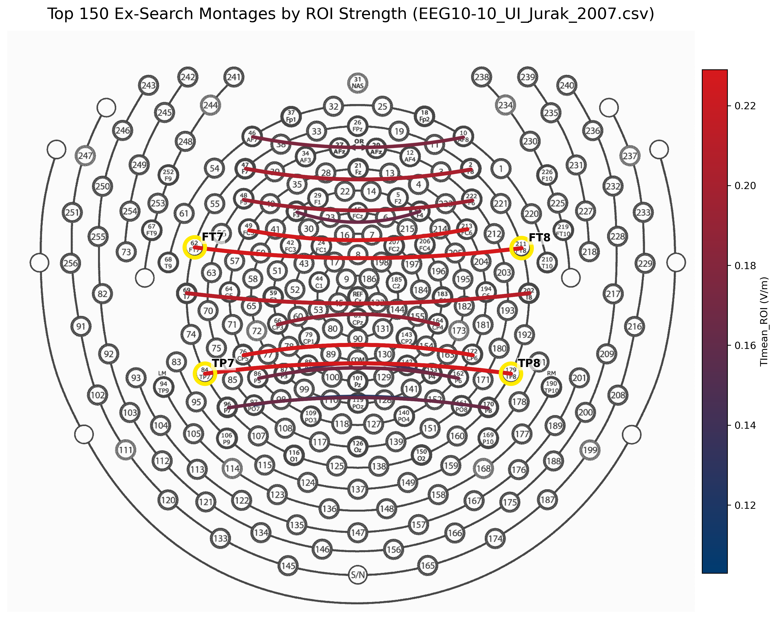Top bilateral montages by ROI strength

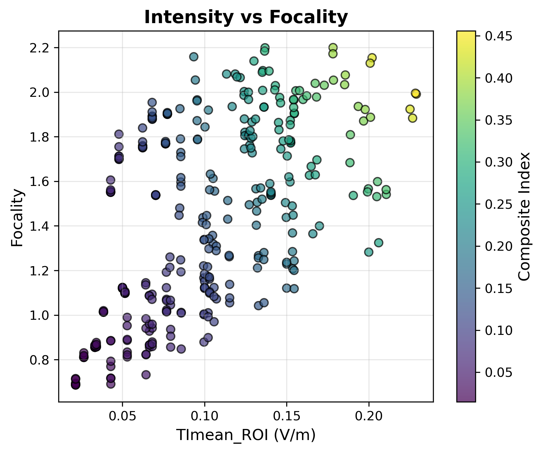Intensity vs focality, 343 evaluations

---

Multipolar (mTI) Mode

Set Search Mode to mTI (4-pair) to run a multipolar exhaustive search (mex-search) instead of the standard two-channel one. tit/opt/mex/ extends ex-search to four channels (eight electrodes), scored with the same verified get_TI_vectors envelope used by the simulator — explicitly not a recursive envelope-of-envelopes (see Envelope Math on the Analyzer page for the \(K\)-carrier modulation-depth math, and Multipolar Mode on the Simulator page for how mTI montages are detected and simulated). The public API is run_m_ex_search(config: MExConfig) -> MExResult, re-exported from tit.opt alongside run_ex_search/run_flex_search.

mTI in the Optimizer

Choose the Ex method for a job row, open its settings and select 8 electrodes (mTI) under Electrodes → Count. The default 4 electrodes (TI) uses two channels. Selecting mTI:

• Uses eight electrode-bucket selectors, E1+ .. E4-, populated from the selected EEG net. mTI is bucket-only; all-combinations mode is available for TI only.
• Switches the current-configuration panel to a Pair Current (mA) spinbox — the per-channel current (range 0.1-10.0, default 2.0, step 0.1) — and a Force left/right symmetry checkbox (unchecked by default) that enables a symmetry-pairing combo — “Within each pair” / “Cross pairs (E1<->E3, E2<->E4)” — once checked.
• Disables the Combine ROIs checkbox only. Saved spherical, atlas-region and imported-mask targets remain available: MExConfig carries roi_names and roi_atlas exactly as ExConfig does, so an mTI run can target a sphere, an atlas region, or an atlas region alone. Combining stays TI-only because the multipolar run path processes selected spheres one at a time.
• Submits a mex job through the shared run controls. Follow its Terminal log or stop it from Jobs.

Candidate enumeration

• Bucket mode (default): the full Cartesian product of the eight buckets, keeping only tuples where all 8 electrode names are distinct (len(set(electrodes)) == 8).
• Pool mode (PoolElectrodes, all_combinations=True): itertools.permutations(pool, 8). A pool of exactly 8 electrodes yields \(8! = 40{,}320\) candidates.
• Symmetric bucket search (symmetric_bucket=True, bucket mode only): restricts candidates to those whose channels mirror left/right, using a mirror map built from an EEG-position CSV (reflecting the x-coordinate across the midline). Two pairing schemes:
  • within_pairs (default): each channel’s own +/- electrodes must mirror each other.
  • cross_pairs: additionally requires channel 1 <-> channel 3 and channel 2 <-> channel 4 to mirror.

  This collapses the search space roughly to linear in bucket size instead of the full Cartesian product.

Scoring

For each candidate, the engine computes four leadfield fields via TI.get_field([e_a, e_b, current_mA/1000.0], leadfield, idx_lf) (mA converted to A), takes vectors = get_TI_vectors(fields), and scores np.linalg.norm(vectors, axis=1). Per-candidate metrics are the same as two-channel ex-search (Metrics above), keyed with the ROI-name prefix ({roi}_TImax_ROI, {roi}_TImean_ROI, {roi}_TImean_GM, {roi}_Focality — 0.0 if the GM mean is \(\le 0\) — and {roi}_n_elements), plus current_ch1_mA .. current_ch4_mA (all four set to the same current_mA). If the ROI has zero elements, all four metrics are 0.0. ROI resolution (spherical CSV centers, NIfTI/MGZ masks, atlas label selections) is inherited wholesale from the ex-search engine.

Outputs

mex-search reuses ex-search’s output pipeline, writing the same file set to derivatives/SimNIBS/sub-{id}/m-ex-search/{run_name}/:

• run_config.json — subject_id, roi_name, roi_radius, leadfield_hdf, electrode_mode ("pool" or "bucket"), electrodes, n_combinations, run_name, current_mA.

• final_output.csv — one row per evaluated candidate, in enumeration order (not sorted). Fixed 8-column header: Montage, Current_Ch1_mA, Current_Ch2_mA, TImax_ROI, TImean_ROI, TImean_GM, Focality, Composite_Index. Currents are formatted to 1 decimal, metrics to 4. The Montage cell strips the TI_field_/.msh wrapper from the candidate key and replaces _and_ with <>.

  Note: the engine computes current_ch3_mA/current_ch4_mA too, but the CSV header has no columns for them — only Ch1/Ch2 currents are recorded (both ex-search and mex-search share this fixed-width CSV writer).

• The same five figures as two-channel ex-search (montage_distributions.png, intensity_vs_focality_scatter.png, and the three EEG-map figures at dpi=300), with four arcs per candidate on the montage maps; regenerate for an existing run with simnibs_python -m tit.opt.ex.results <run_dir>.

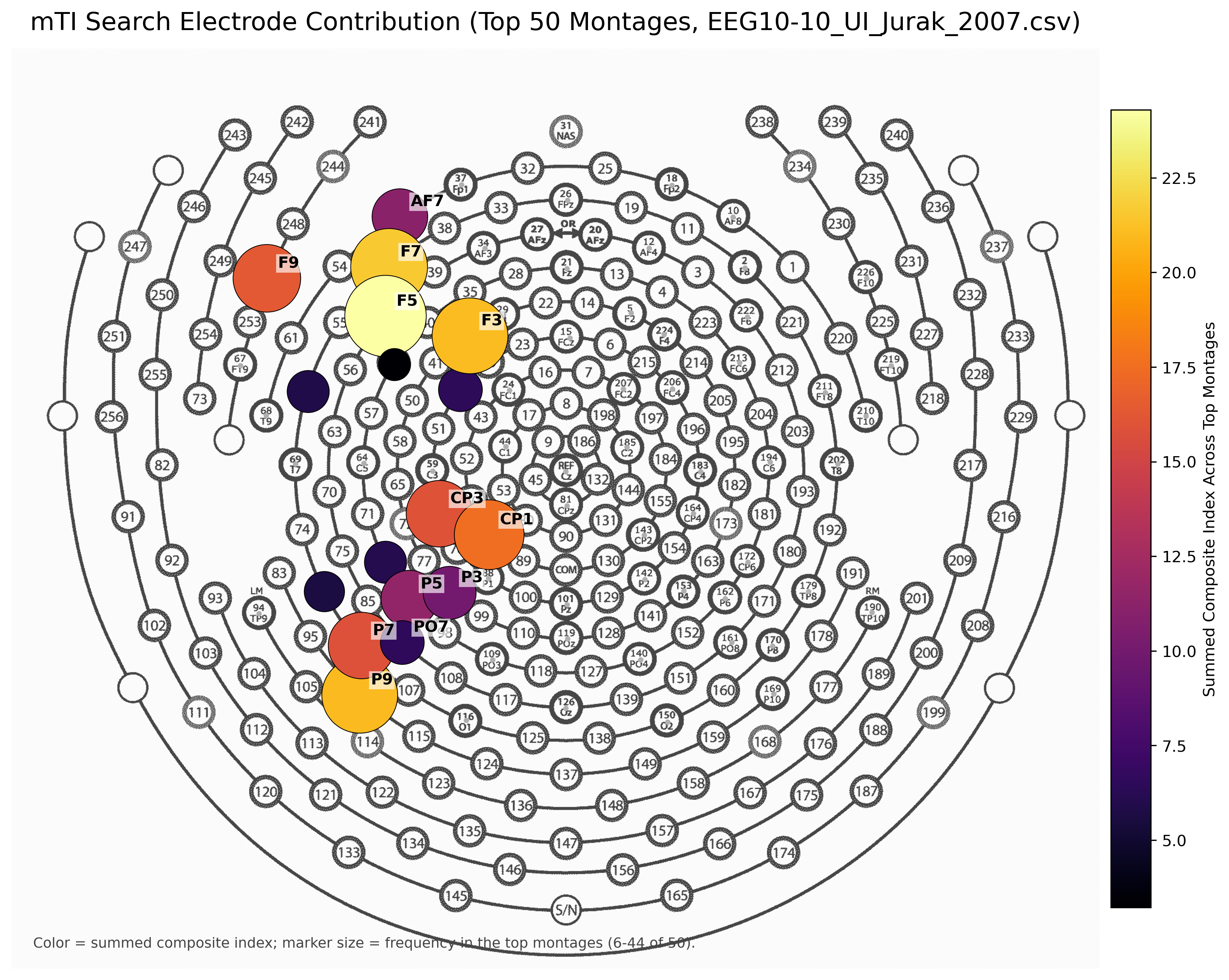
electrode_score_heatmap.png, 576-candidate run

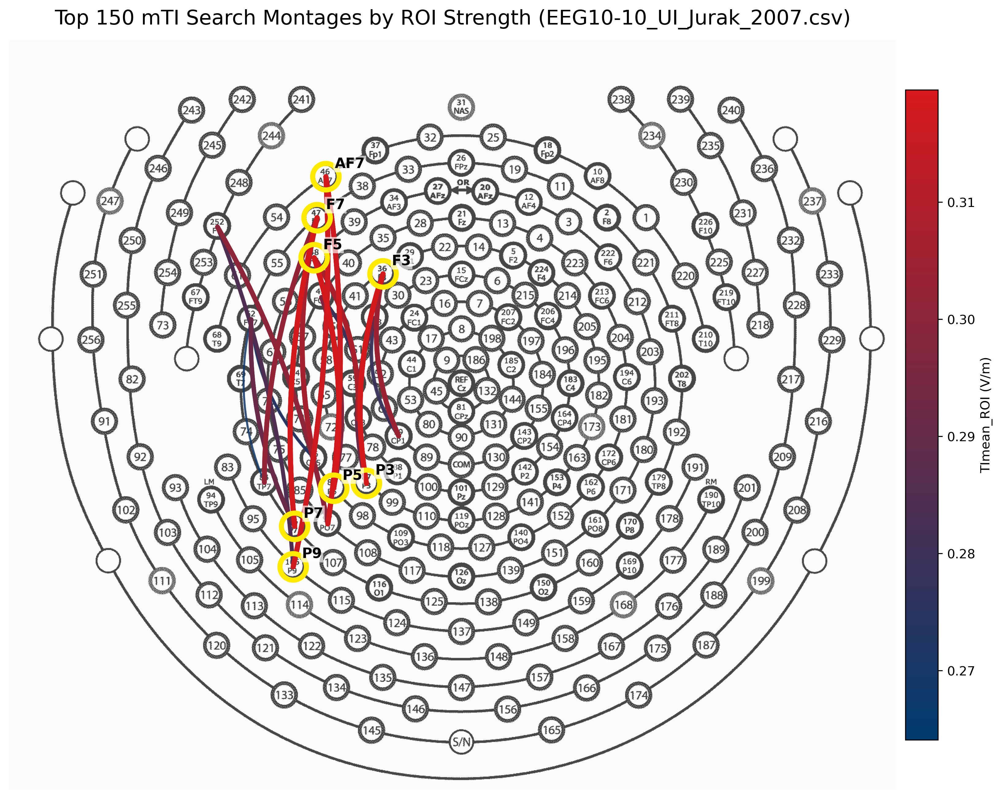
montage_strength_map.png, four arcs per candidate

The candidate key/name format is TI_field_{e1a}_{e1b}_and_{e2a}_{e2b}_and_{e3a}_{e3b}_and_{e4a}_{e4b}_I-{current_mA:.1f}mA.msh — no mesh file is actually written; it is only a label. Progress is logged per candidate plus a coarse estimate every 500 candidates, since bucketed four-channel searches can reach hundreds of thousands of combinations. SIGINT/SIGTERM interruption and the zero-candidate fail-fast behave exactly as in two-channel ex-search.

Example run (sub-ernie, v2.4.0)

Bucket search with 3·3·2·2·2·2·2·2 candidate electrodes for e1_plus … e4_minus → 576 four-channel candidates, Jurak 10-10 leadfield, 5 mm ROI at MNI (−38, 5, 0), current_mA = 1.0. Wall time 13.0 min on 12 cores (1.35 s per candidate with the numba kernel and the worker pool).

Best montages (by Composite_Index)	TImax_ROI	TImean_ROI	TImean_GM	Focality	Composite_Index
F7_P7 <> F5_CP3 <> F3_P3 <> AF7_P9	0.4769	0.3074	0.1571	1.9573	0.6017
F7_TP7 <> F5_CP3 <> F3_P3 <> AF7_P9	0.4754	0.3009	0.1532	1.9641	0.5911
F7_CP5 <> F5_CP3 <> F3_P3 <> AF7_P9	0.4810	0.3043	0.1572	1.9364	0.5893
F7_P7 <> F5_P5 <> F3_CP1 <> F9_PO7	0.4699	0.3017	0.1568	1.9239	0.5804

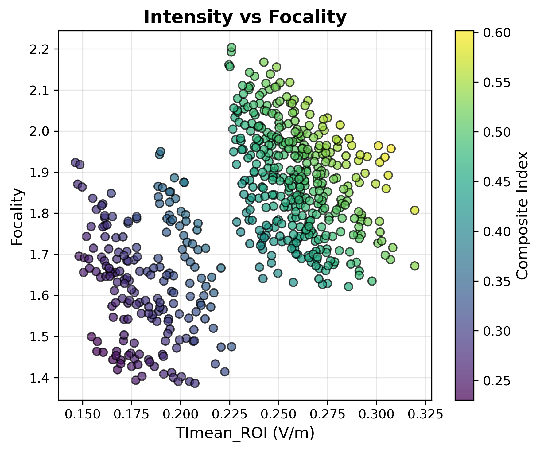
intensity_vs_focality_scatter.png: the 576 candidates trace the intensity–focality trade-off; the isolated low-intensity cluster on the left is the T7-anode family, the frontier on the upper right is where the Composite_Index maximum sits.

Symmetric (bilateral) search. With symmetric_bucket: true and symmetry_pairing: "within_pairs" only left/right-mirrored channels are enumerated: each channel’s minus electrode must be the mirror of its plus electrode (F7–F8, CP5–CP6, …), so the buckets are written as left candidates in e{k}_plus and their mirrors in e{k}_minus. Five bilateral candidates per channel → 5⁴ = 625 candidates, 13.9 min (1.33 s each):

Best bilateral montages	TImax_ROI	TImean_ROI	TImean_GM	Focality	Composite_Index
F7_F8 <> CP5_CP6 <> F1_F2 <> PO7_PO8	0.3910	0.2103	0.1074	1.9577	0.4117
F7_F8 <> CP5_CP6 <> F1_F2 <> P9_P10	0.3920	0.2102	0.1073	1.9584	0.4117
F5_F6 <> CP5_CP6 <> F1_F2 <> PO7_PO8	0.3915	0.2085	0.1057	1.9722	0.4113

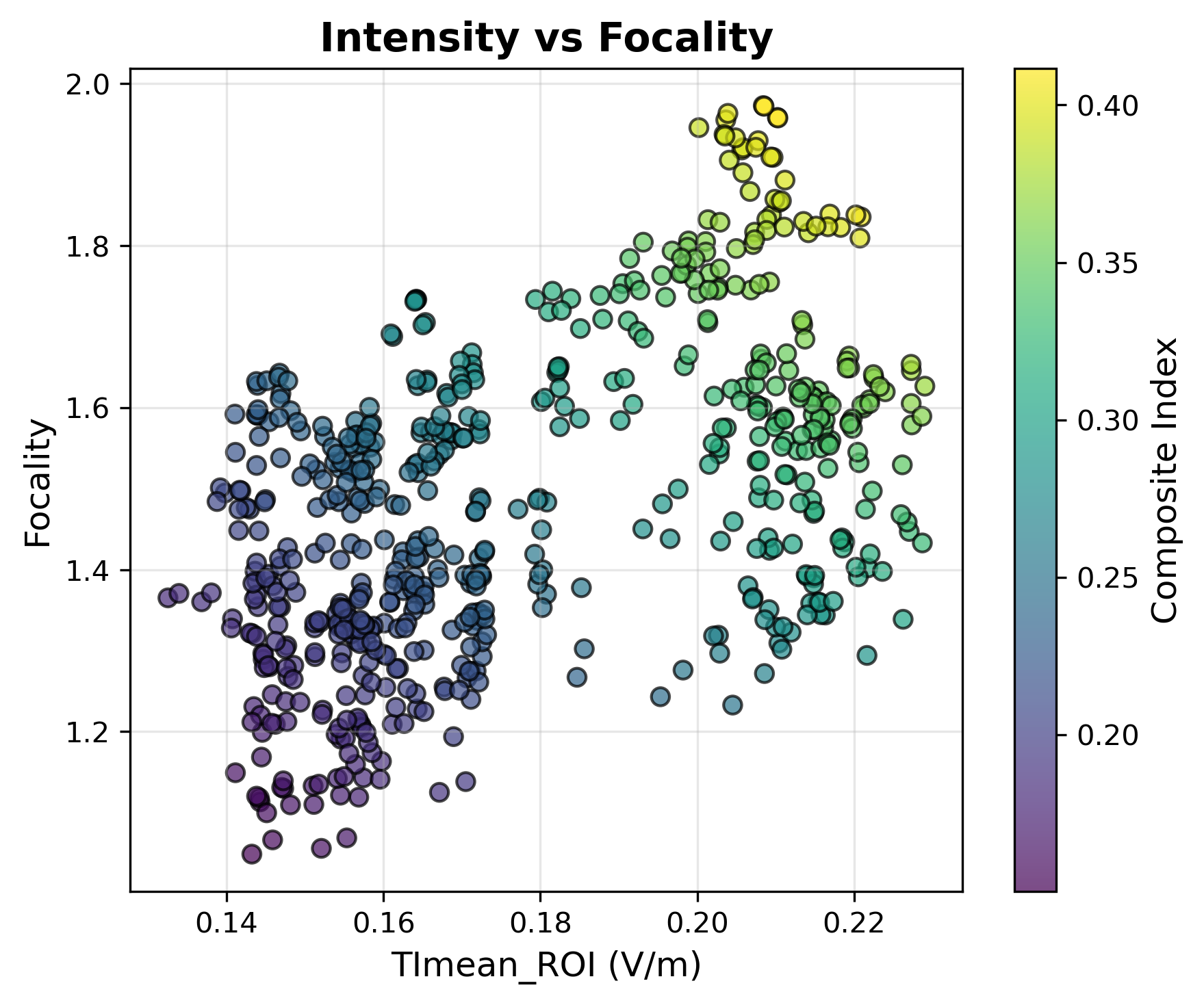
Bilateral montages reach ~⅔ of the ROI intensity of the unconstrained search for this left-lateral target (0.21 vs 0.31 V/m at similar focality) — the expected price of symmetry; symmetry_pairing: "cross_pairs" additionally mirrors channels 1↔3 and 2↔4.

Cost. Scoring one four-channel candidate with the verified multi-carrier envelope is a per-element direction search (192-direction sweep plus local refinement), not a closed form like two-channel ex-search. The search is evaluated on ROI ∪ GM only by a fused numba kernel (tit/_mti_kernel.py, sharing the job’s CPUs with the workers) and candidates are distributed over forked worker processes (n_jobs, default the global CPU limit, 70 % of the cores): on a 12-core machine this is ~1–2 s per candidate, i.e. a few hundred candidates in ~10 min. The first call pays ~10 s of JIT compilation, cached afterwards. There is no current-ratio sweep in mex-search; each run uses a single current_mA.

Running it

simnibs_python -m tit.opt.mex config.json

JSON config keys: project_dir, subject_id, leadfield_hdf, roi_name, electrodes (_type: "BucketElectrodes" or "PoolElectrodes", plus e1_plus..e4_minus or electrodes), current_mA, roi_radius, roi_names, roi_atlas, roi_coordinate_space, run_name, n_jobs (worker processes, default −1 = the global CPU limit; larger values are capped at it), symmetric_bucket, symmetry_eeg_csv, symmetry_pairing.

{
  "project_dir": "/path/to/project",
  "subject_id": "101",
  "leadfield_hdf": "101_leadfield_EEG10-20_Okamoto_2004.hdf5",
  "roi_name": "L-Insula.csv",
  "electrodes": {
    "_type": "BucketElectrodes",
    "e1_plus": ["Fp1", "Fp2"],
    "e1_minus": ["Pz", "Oz"],
    "e2_plus": ["C3", "F3"],
    "e2_minus": ["C4", "F4"],
    "e3_plus": ["T7", "T8"],
    "e3_minus": ["O1", "O2"],
    "e4_plus": ["Fz", "Cz"],
    "e4_minus": ["P3", "P4"]
  },
  "current_mA": 2.0,
  "roi_radius": 3.0
}

The multipolar exhaustive search combination logic (tit/opt/mex/logic.py) and the generalized electrode-bucket loader (tit/opt/ex/buckets.py) were ported from collaborator Larissa Albantakis’s branch alba/ex-search-multipolar.

Target preview

The Scene pane displays the selected mask, subcortical regions, or saved ROI spheres in subject space. It is read-only: edit targets in the job form. Multiple saved ROIs are shown together; the Combine setting still determines whether they run together or separately. The preview shows target extent before search-specific tissue and mesh filtering.