Gallery
A film of the viewer in use, then 49 plates of what it renders — brain MRI and head models, head/chest/abdomen CT, abdominal and spinal MRI, and the segmentations that go with them. Every frame and every plate is rendered offscreen by the same engine the window uses, from a job document in docs/screenshots/2026-08-29/jobs/; the datasets and their licences are listed in docs/TESTING.md.
The film
A 108.7-second tour of the interface and the rendering engine, over the real sub-ernie SimNIBS dataset. Neither the video nor the GIF is hand-edited: examples/capture/showcase.py writes six job documents, the app renders every frame offscreen through the same Engine calls a user makes with the mouse (see Automation & Python), and ffmpeg joins them and burns the captions. Capture guidance is in docs/AUTOMATION.md; the script owns the shot list and timings.
For anywhere a <video> tag doesn't reach, the same tour as a GIF — 7.9 MB, so it is loaded only when it is scrolled to:

The plates
Hero
The pictures the home page and README lead with — one scene per data domain.
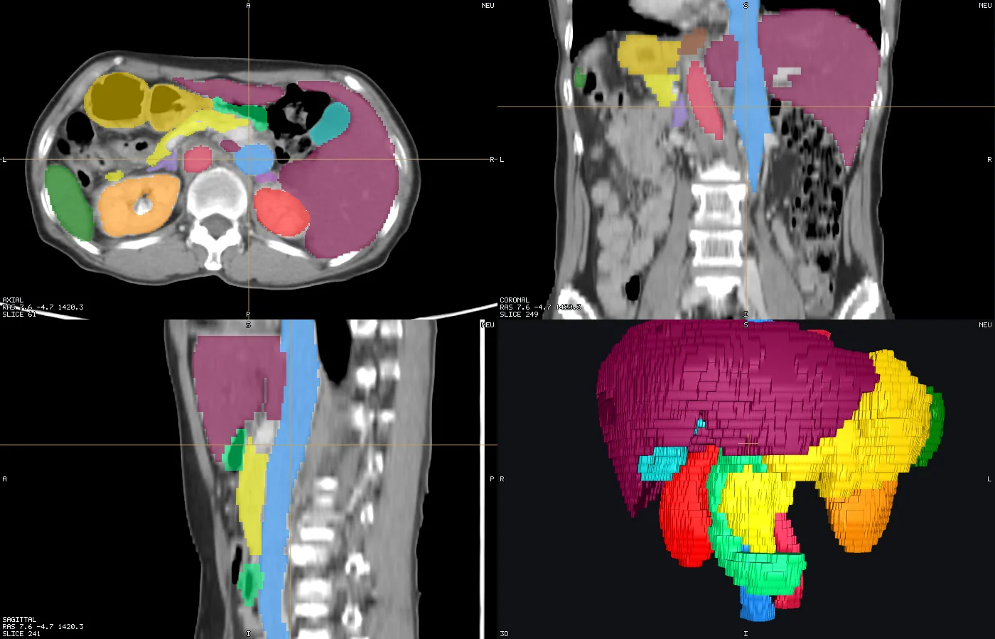
Abdominal CT with organ labels
A 2x2 of an abdominal CT in a soft-tissue window (W400/L40) with the 15 AMOS organ labels filled at 0.55, the crosshair driving all three planes, and the organs as marching-cubes surfaces in the 3D pane.
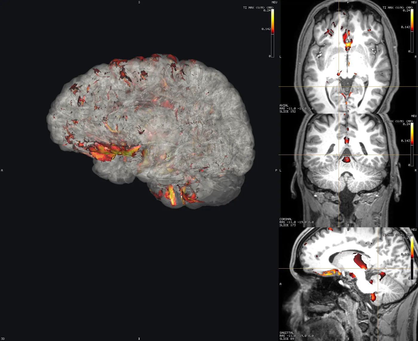
A simulated field in the brain
The TI_max field of a thalamic montage, thresholded at its own 90th percentile with the scale running p90 -> p97 -> p99.9: in the big 3D pane of a 1+3 layout the field on grey_Thalamus_TI.msh inside a translucent grey-matter surface, seen 30 degrees off left-lateral; in the slice panes the same field as a localised heat overlay on the T1. One colour bar.
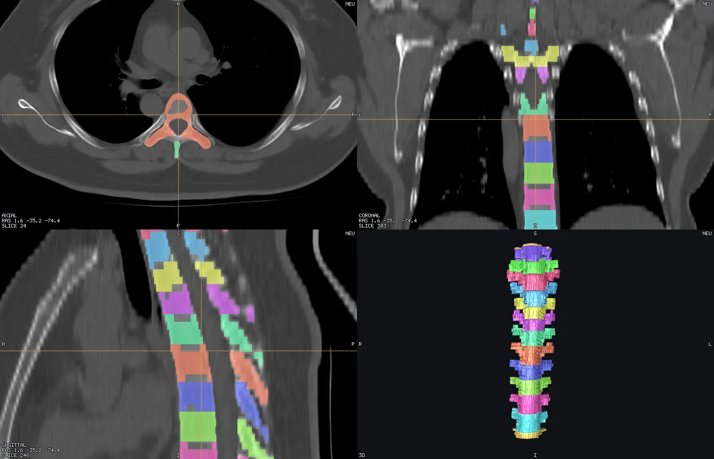
Chest CT with per-vertebra labels
A 2x2 of a chest CT in a bone window (W1500/L300) with every vertebra separately labelled, and the whole labelled column rebuilt as one surface per vertebra in the 3D pane.
Brain
The SimNIBS head model the viewer was built around: the T1, its surfaces, atlas and electrodes, the tissue mesh, and simulated tES fields on it.
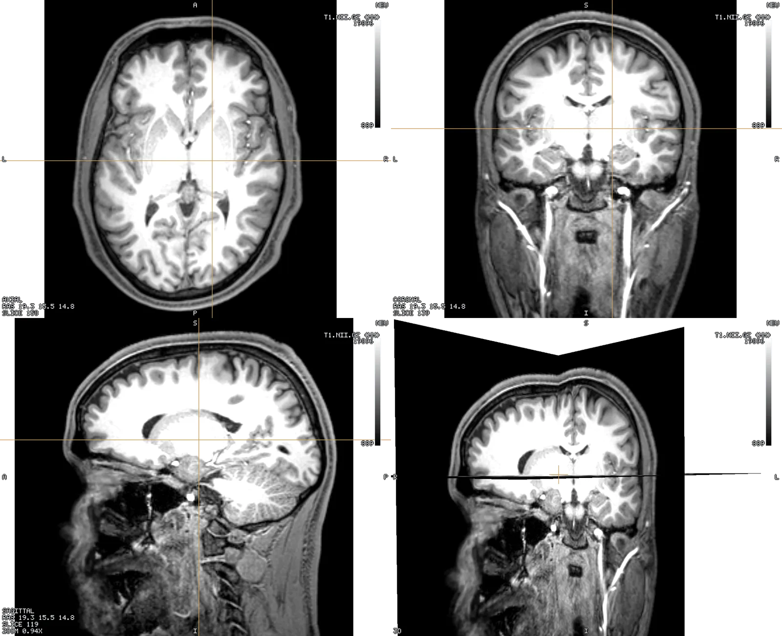
T1, four panes
The subject's T1 in the 2x2 layout: axial, coronal and sagittal slices through one crosshair, and the three planes standing in the 3D pane.
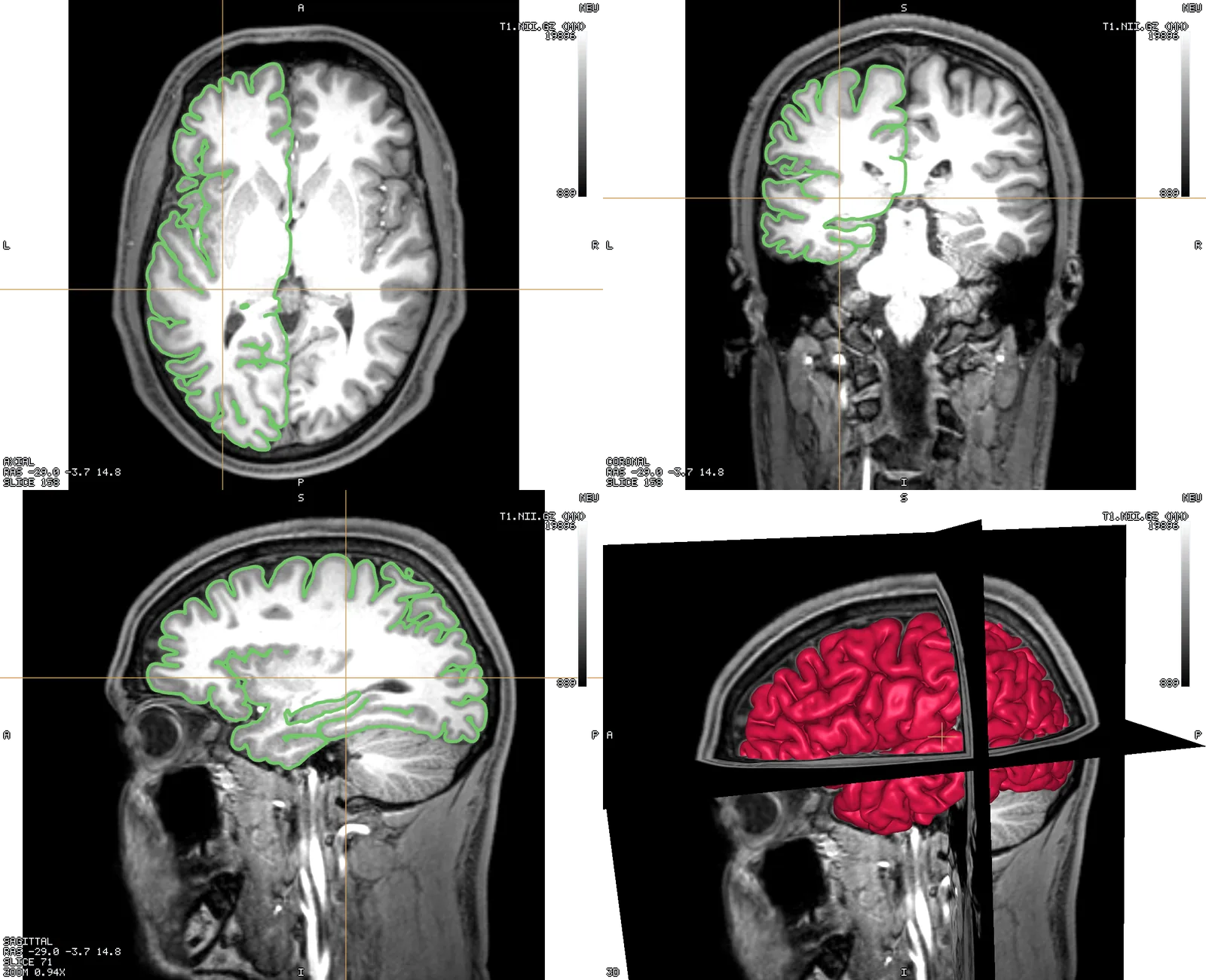
T1 with the left pial surface
lh.pial.gii as a green contour wherever it crosses a slice, and the surface itself among the T1's planes in the 3D pane.
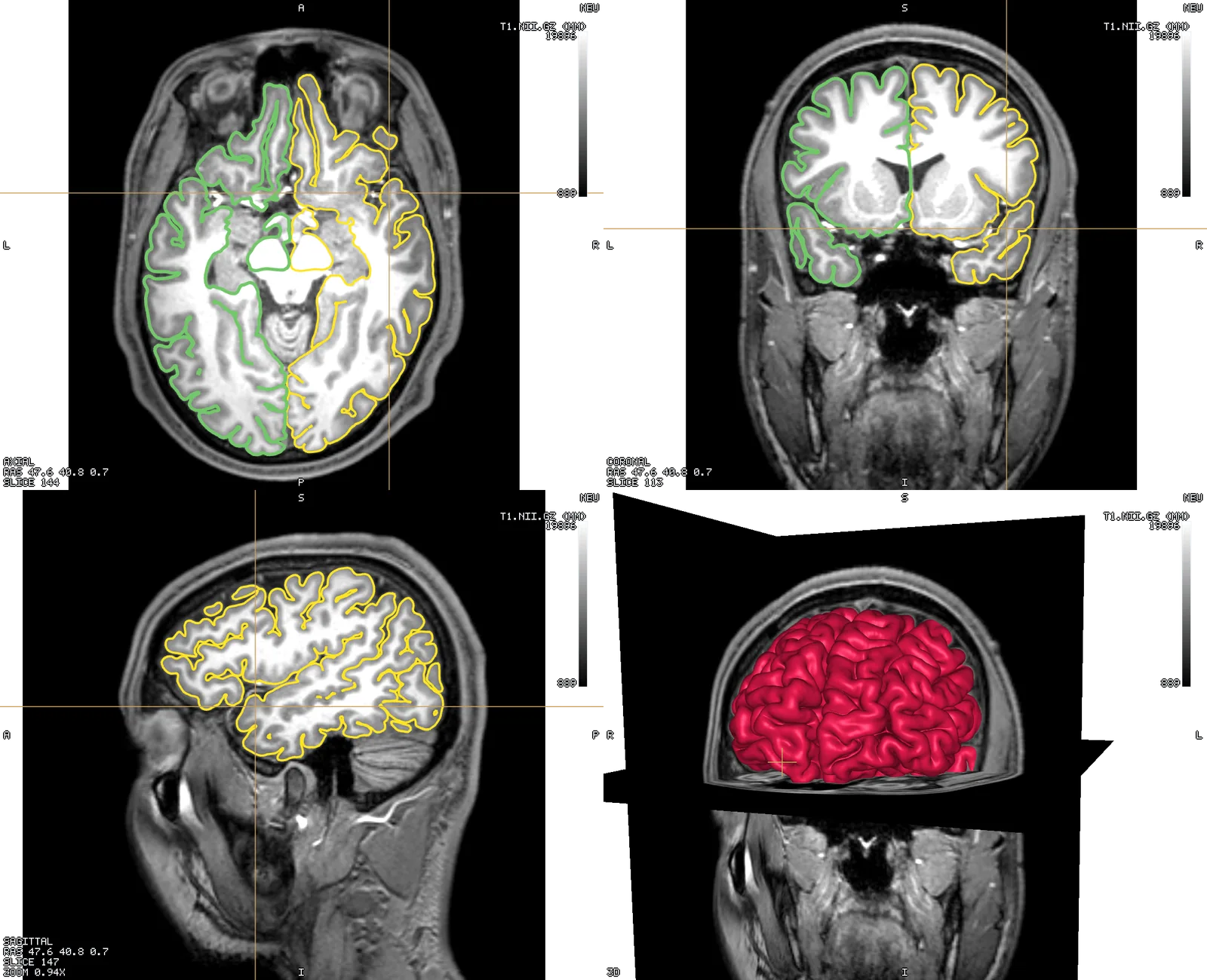
T1 with both pial surfaces
Left and right pial surfaces as contours in the slice panes (green and yellow), and both hemispheres in 3D, seen from the left with the axial plane cut below them.
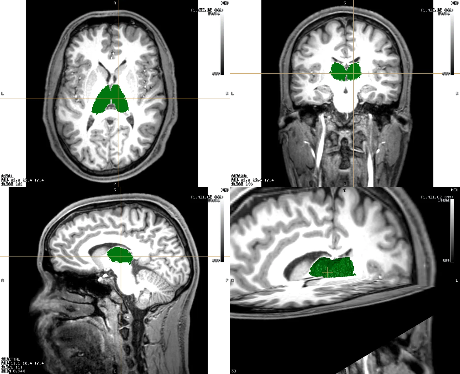
The thalamus, soloed
The labeling atlas reduced to the left and right thalamus (ids 10 and 49) filled at full opacity over the T1, and the same region as a 3D surface between the slice planes, close up.
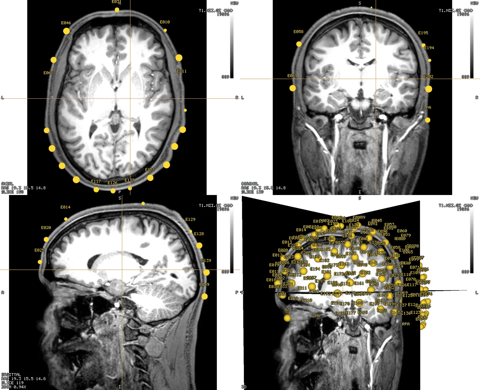
EEG electrodes on the T1
A 185-channel HydroCel net read from a Gmsh .geo view: labelled spheres wherever an electrode sits on a slice, and the whole net over the head in 3D.
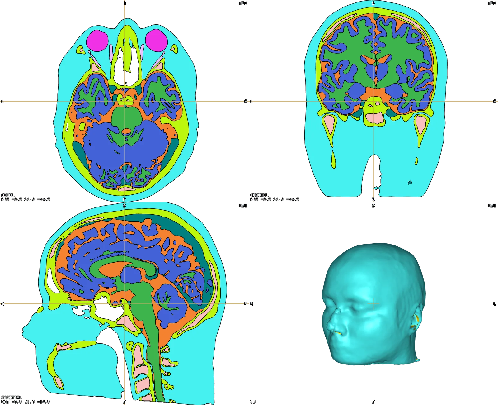
Tissue segmentation with the head mesh
final_tissues.nii.gz filled at full opacity in its SimNIBS LUT colours, 2x2, with the head mesh's scalp surface alone in the 3D pane.
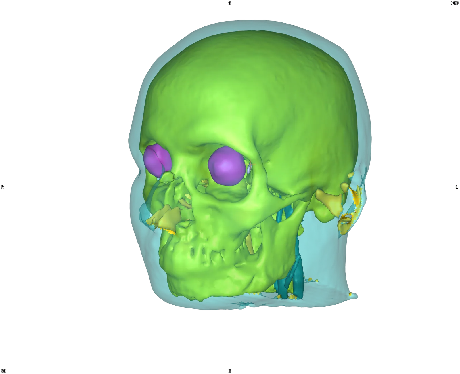
Skull through a translucent scalp
ernie.msh in 3D with the scalp at low opacity over the opaque skull, eyes and the paranasal sinuses, from an anterior-oblique camera.
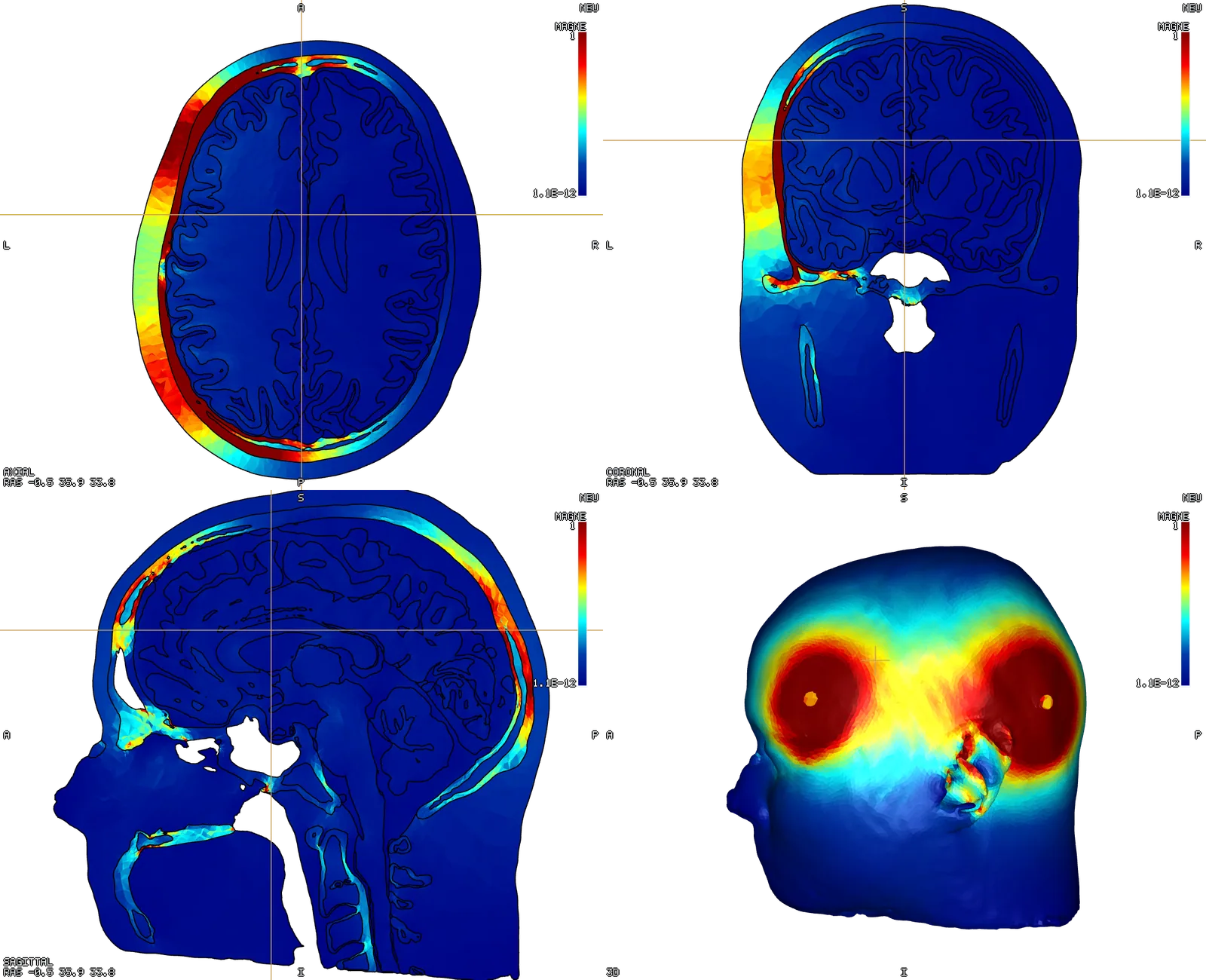
A tDCS field on the whole head mesh
|E| of a tDCS simulation painted on every tissue of the head mesh: the 2D cuts filled by the field with the tissue boundaries outlined, and the scalp in 3D showing the two electrodes as the hot spots.
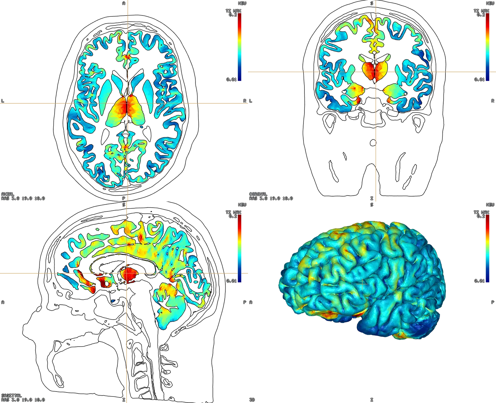
TI_max on the grey matter
The grey-matter mesh of a thalamic TI montage coloured by TI_max on a jet scale from 0.01 to 0.2 V/m: the cortex cut by the three slices in 2D and the whole surface in 3D, one colour bar.
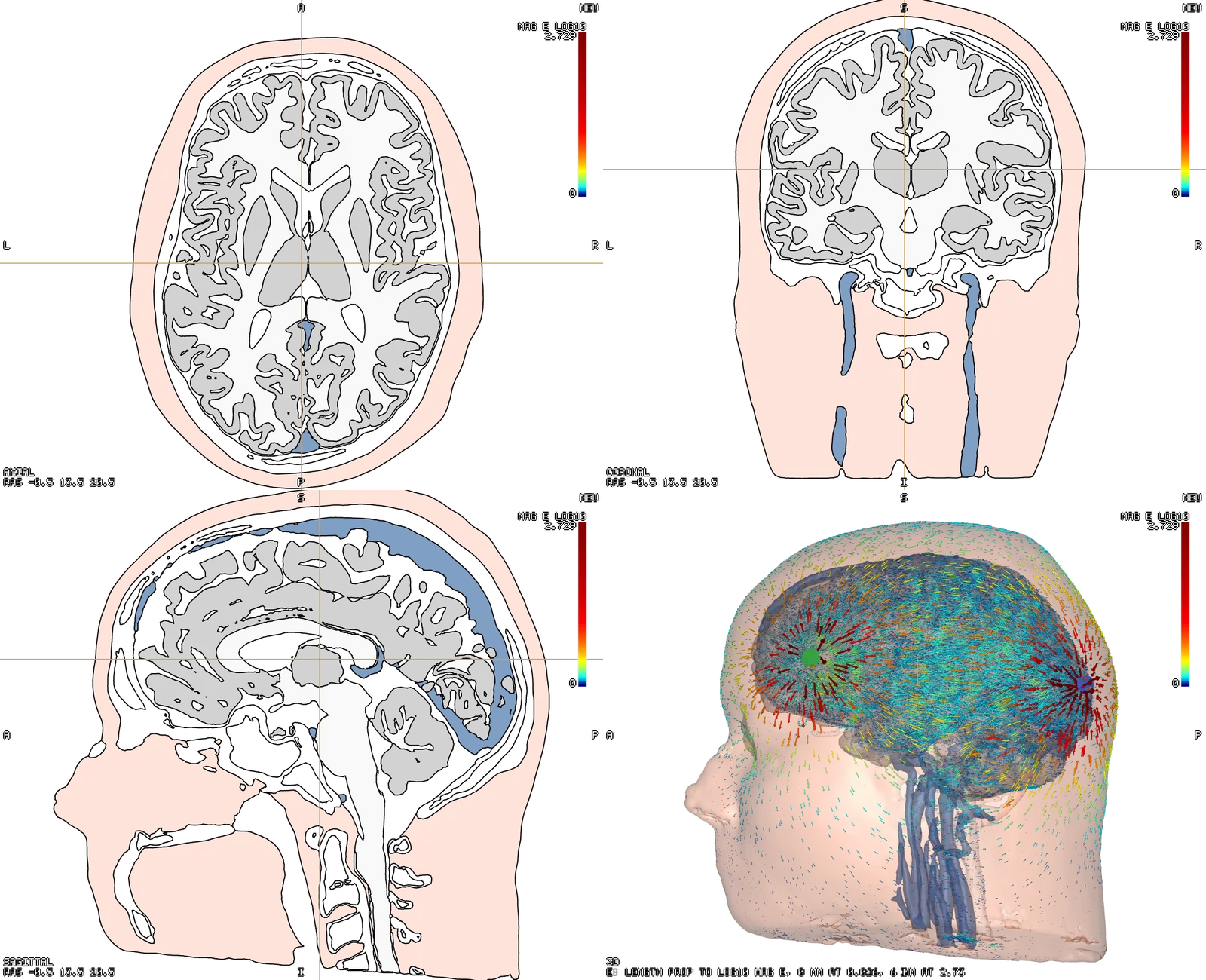
The E vector field as glyphs
The tDCS mesh with its tissues in flat colours in the slice panes, and in the 3D pane the E field as arrows coloured by magnitude and log-scaled in length, over a translucent scalp.
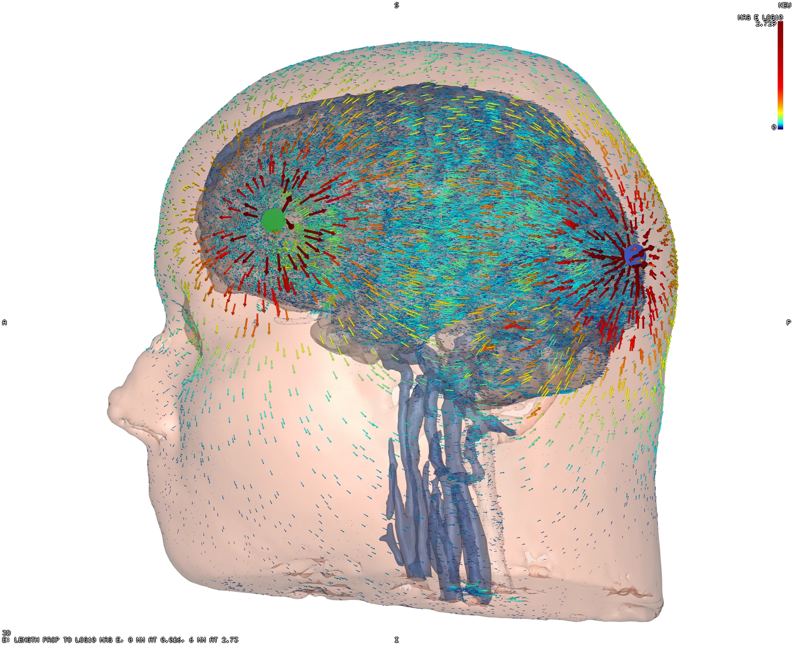
E-field glyphs, 3D alone
The same glyphs filling a single 3D pane from the left: the field radiating from the two electrodes, red near them and blue deep in the head.
Modalities
Nothing in the viewer is head-specific. The same build, controls and job runner across MRI, CT and segmentations of the head, chest, abdomen, spine and pelvis — each dataset as the plain contrast and then with the segmentation that came with it.
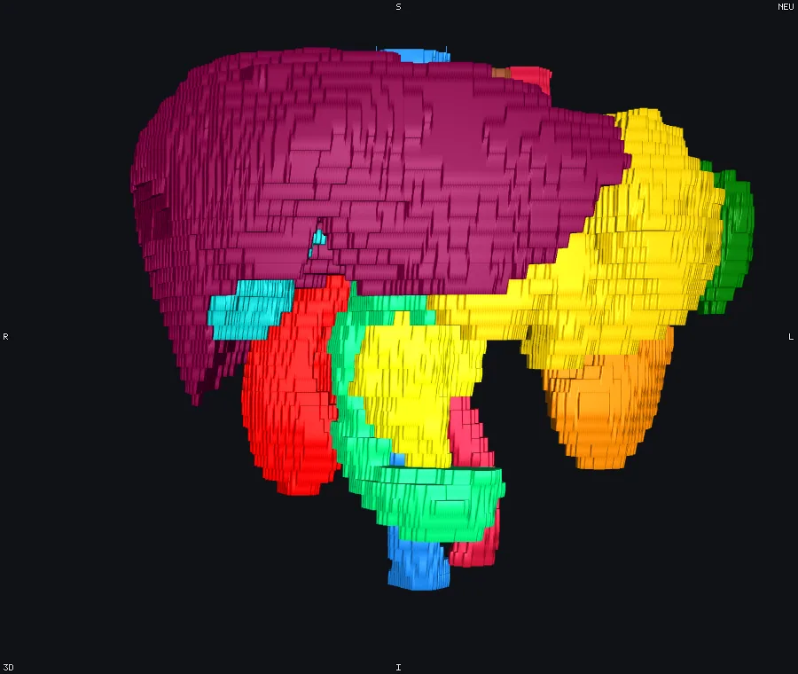
Abdominal organs as surfaces
The thoraco-abdominal organs (labels 1-13) as one isosurface per region, anterior camera.
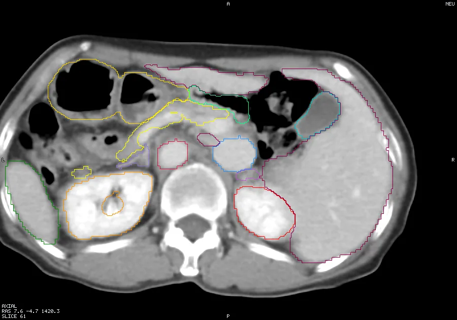
Abdominal CT with organ outlines
The same slice with the organ label map in outline mode at full opacity — the anatomy stays readable under the segmentation.
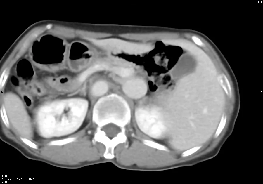
Abdominal CT, soft-tissue window
One axial pane at W400/L40 through the kidneys and pancreas, framed to the patient rather than to the scanner bore.
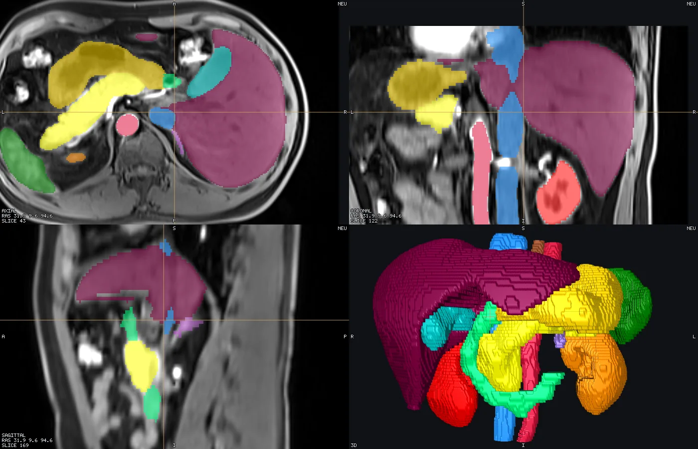
Abdominal MRI with organ labels
A 2x2 with the 13 organ labels filled at 0.55 and the organ surfaces in 3D: the same segmentation workflow on MRI as on CT.
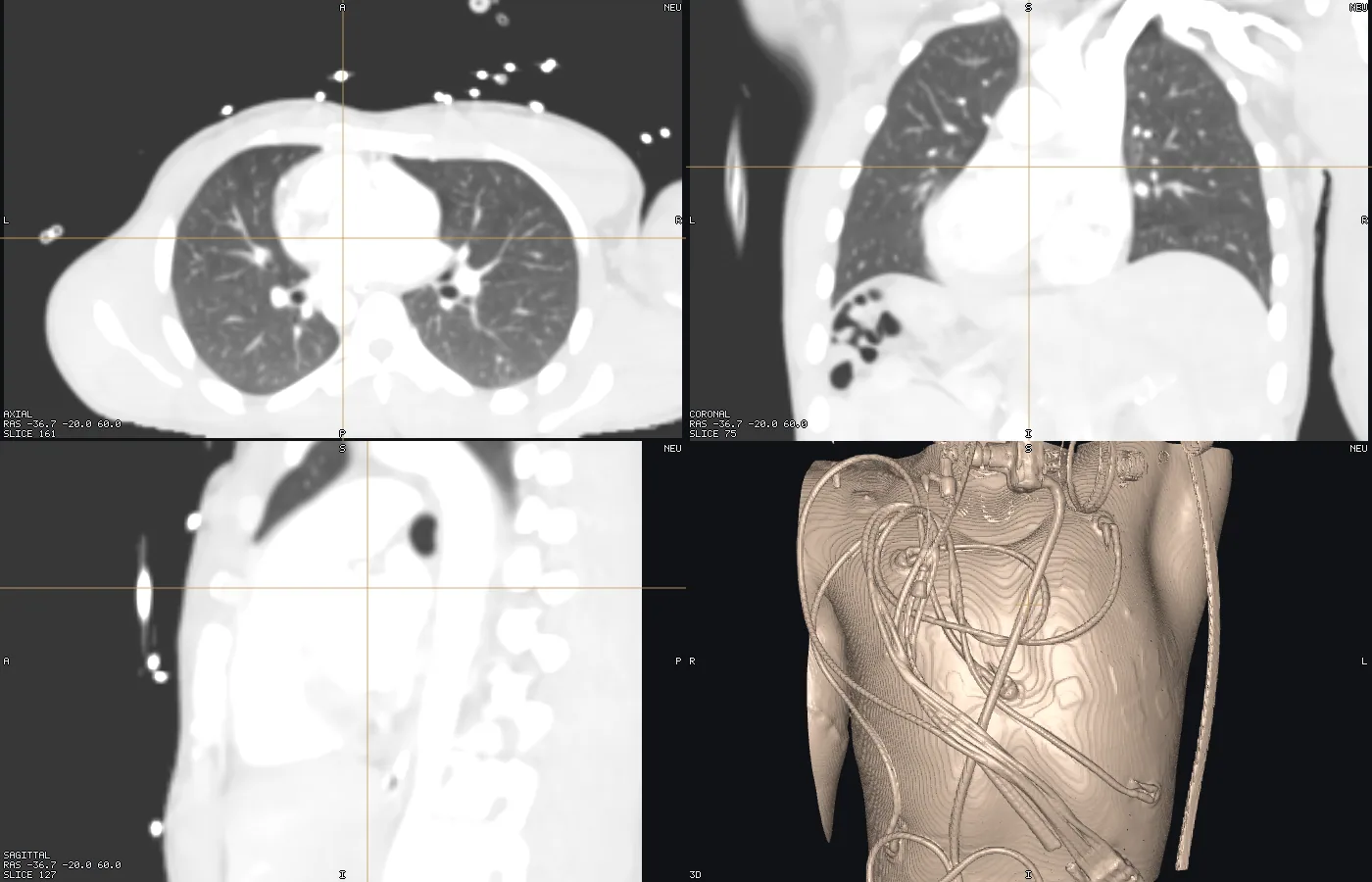
Chest CT, lung window
The same scan in three planes at W1500/L-600, plus the body surface as an isosurface of the CT at -300 HU in the 3D pane — the ECG leads and lines are on it.
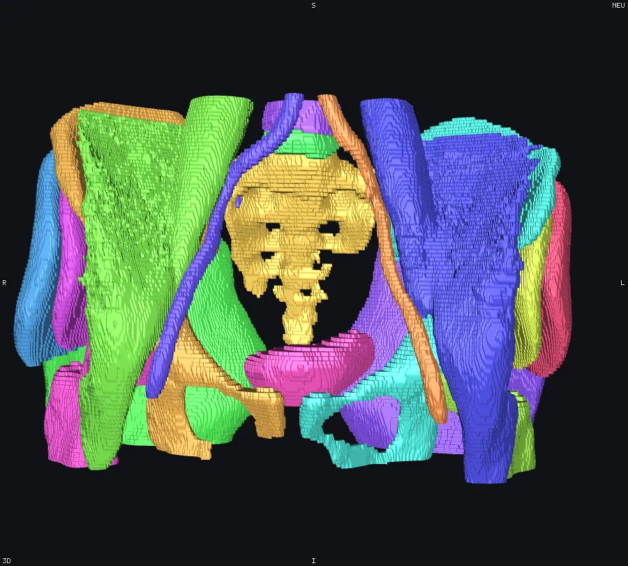
Pelvic structures as surfaces
Hips, femurs, sacrum, vertebrae, bladder, iliac vessels and the gluteal and iliopsoas muscles as isosurfaces, narrowed to 18 of the 26 structures so the set stays readable.
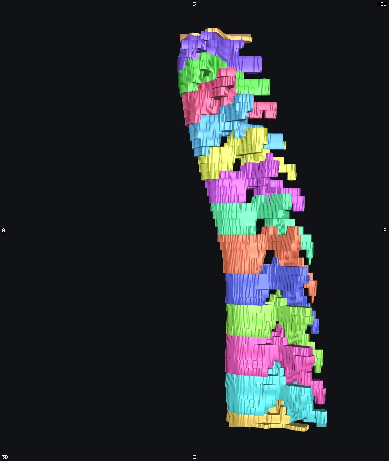
Vertebrae as surfaces
The labelled column rebuilt as one surface per vertebra, seen from the left, so the kyphosis is visible.
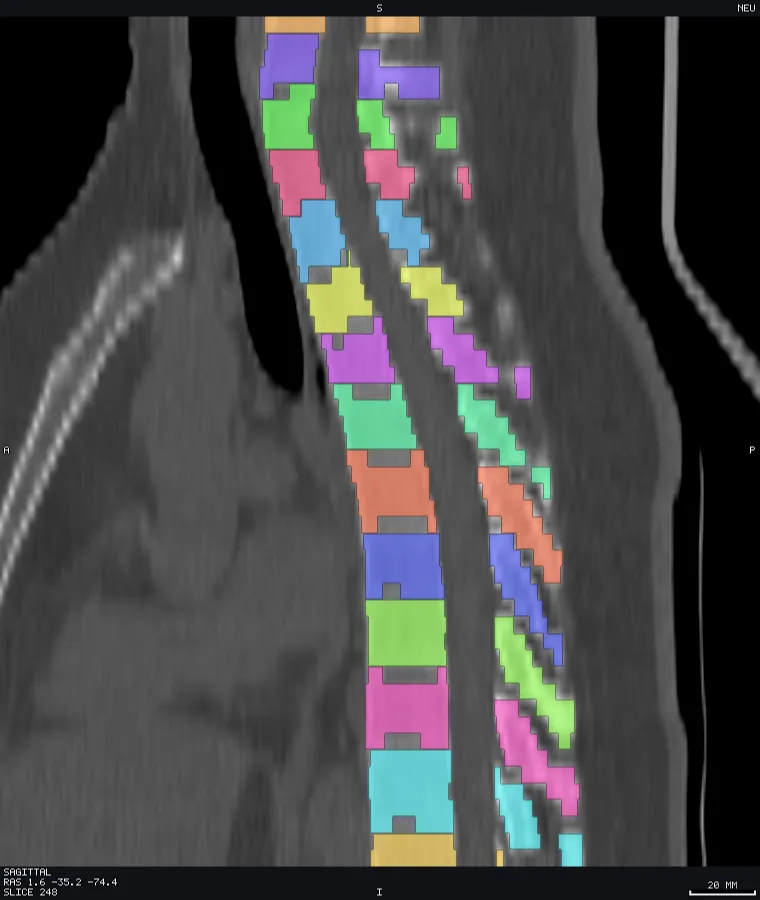
Spine CT with per-vertebra labels
The same pane with the vertebra label map in fill+outline mode at 0.75 — one colour per vertebral level.
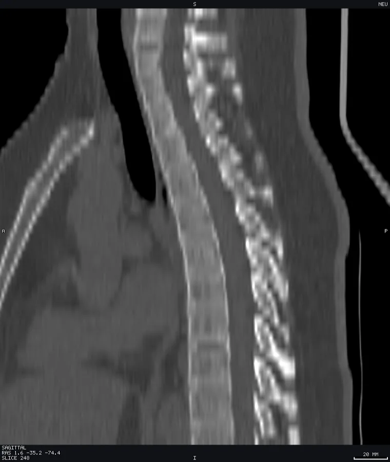
Spine CT, sagittal bone window
A single sagittal pane of the thoracic column in a bone window, with a scale bar.
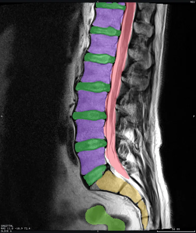
Lumbar spine MRI with labels
The same slice with vertebrae, intervertebral discs, the spinal cord and the sacrum filled at 0.5.
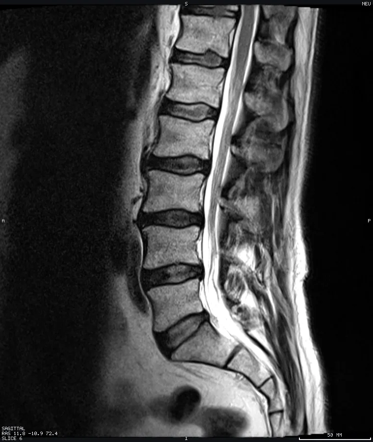
Lumbar spine MRI, sagittal
A sagittal lumbar MRI at 0.34 mm/px with a scale bar — the plain contrast, before any segmentation.
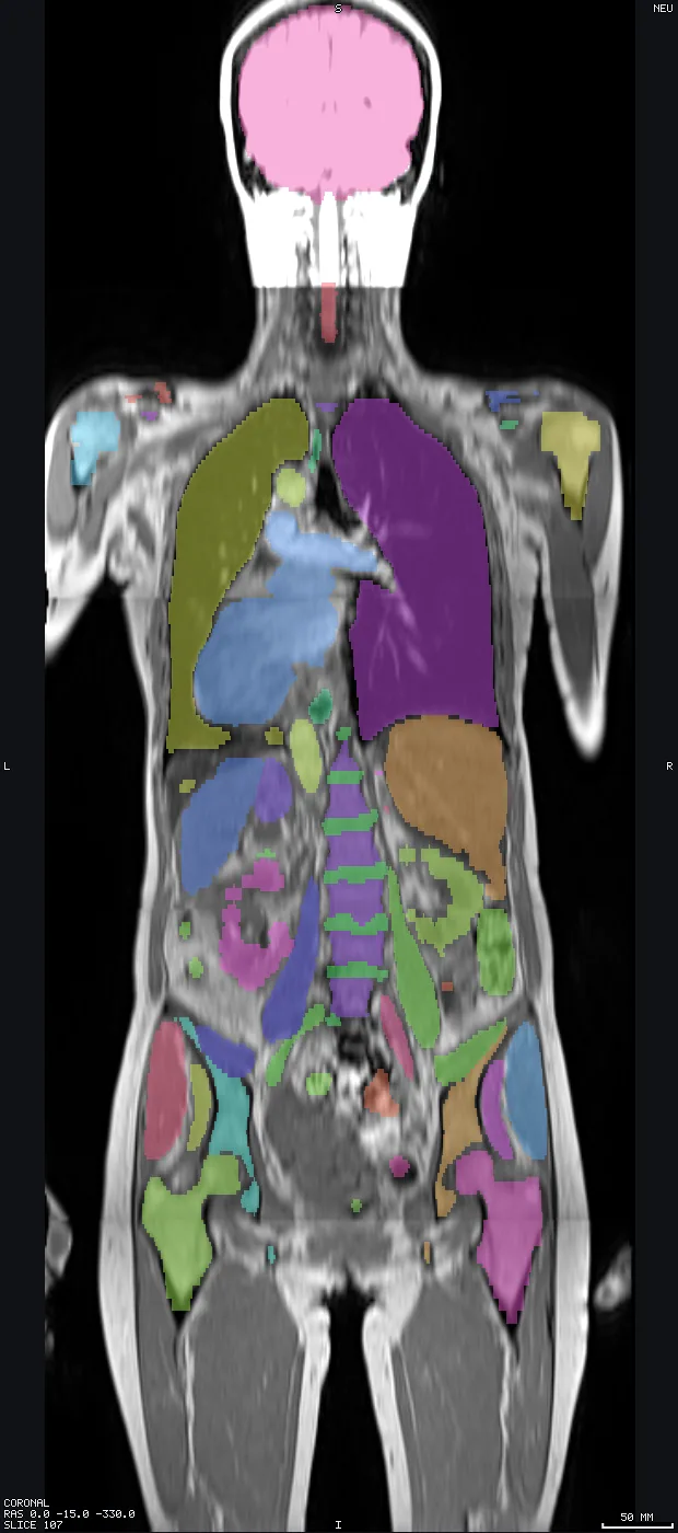
Whole-body MRI with 49 structures
A single coronal pane covering 1,050 mm of subject from the brain to mid-thigh, with all 49 TotalSegmentator-MR structures filled at 0.45 and a scale bar.
Features
One or two plates per section of the guide, so every control has a picture.
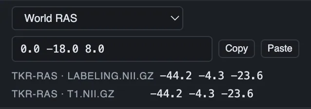
Coordinates and template spaces
The coordinate bar with the space selector on MNI152 (nonlinear) and the TKR-RAS and MNI readouts populated from the subject's toMNI/ warp.
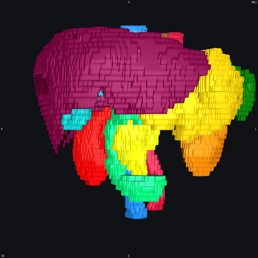
Isosurfaces, off the head
The isosurface feature on a non-brain volume: one marching-cubes surface per organ label of an abdominal CT, no anatomy planes behind them.
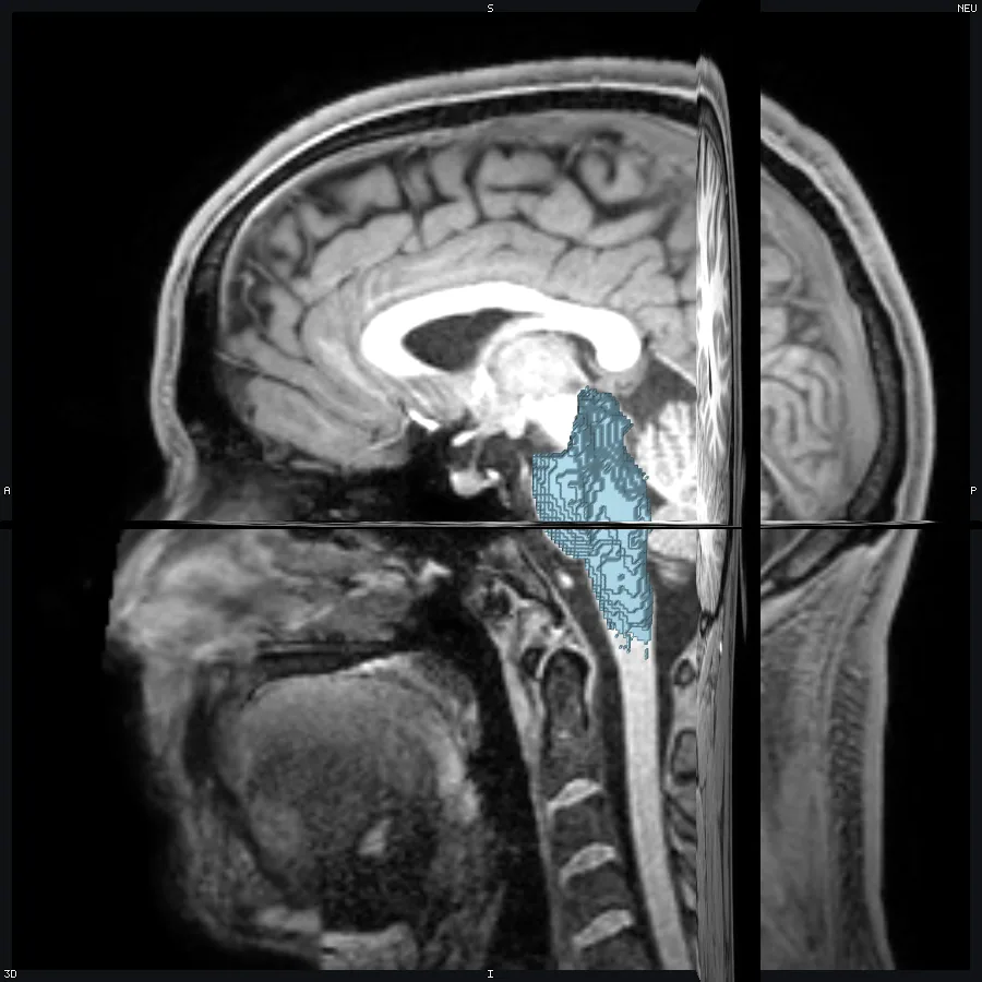
A region as a 3D surface
The brain stem (id 16) built as an isosurface from the label volume, standing among the T1's slice planes.
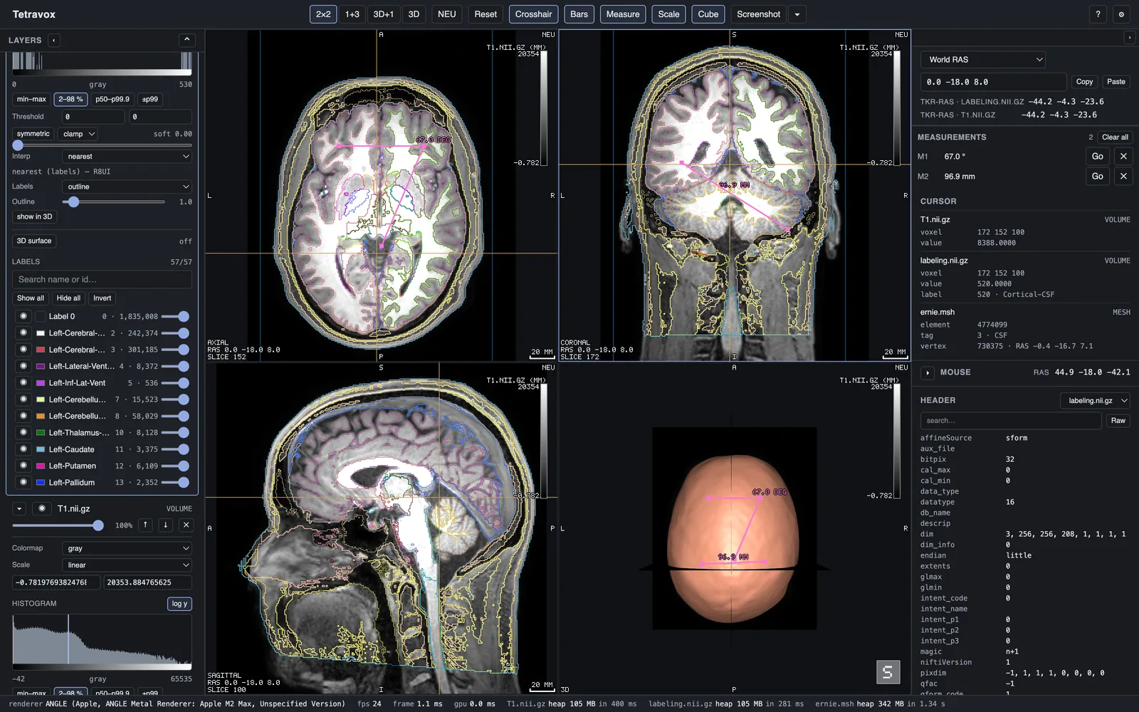
Measurements
An angle in the axial pane and a length in the coronal one, listed in the Measurements panel with Clear all.
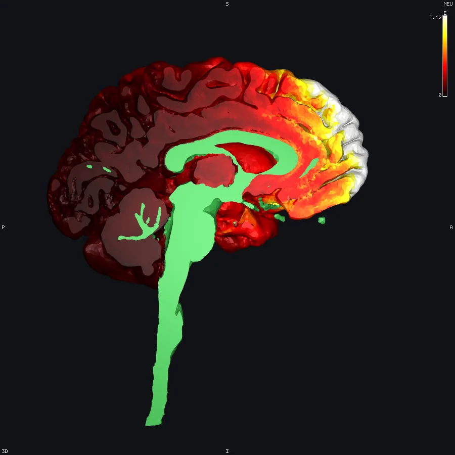
Per-tissue paint
One mesh, two colour sources on a sagittal cut: the grey matter painted by the E-field, the white matter in its own tissue colour.
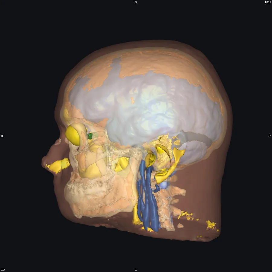
Translucent tissues
The mesh-tissues-translucent preset: scalp at 0.3, skull at 0.5, grey and white matter opaque.
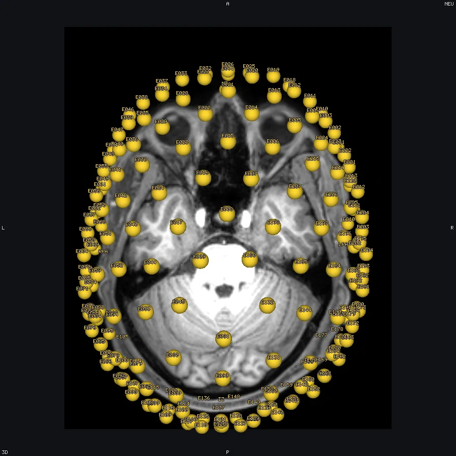
EEG electrode positions
A 185-channel HydroCel montage read from a Gmsh .geo view, labelled, over the T1's slice planes.
Motion
Orbits, slice sweeps and animated parameters, rendered offscreen by the job runner.
A simulated field's threshold
A 2x2 with the grey-matter surface in 3D and a simulated TI field over the T1, its threshold climbing from the field's own p50 (0.081 V/m) to its p97 (0.133 V/m) and falling back. Colour bar on, because a field is on screen. 28 frames at 12 fps, 560 px square; `motion/field-threshold-rise.mp4` is the same clip as H.264.
Abdominal organ turntable
The 13 thoraco-abdominal organ surfaces of an AMOS22 CT turning through 360 deg. 36 frames at 12 fps, 560 px square; `motion/orbit-abdomen-organs.mp4` is the same clip as H.264.
Vertebra turntable
The per-vertebra isosurfaces of a chest CT turning through 360 deg. 36 frames at 12 fps, 560 px square; `motion/orbit-spine-vertebrae.mp4` is the same clip as H.264.
Axial sweep with the atlas
An axial sweep from z = -45 to z = +70 mm with the 41 intracranial atlas labels outlined, and back — inferior to superior and down again, so the loop has no snap. 32 frames at 12 fps, 560 px square; `motion/sweep-axial-t1-atlas.mp4` is the same clip as H.264.
Interface
The window, its panels and its dialogs.
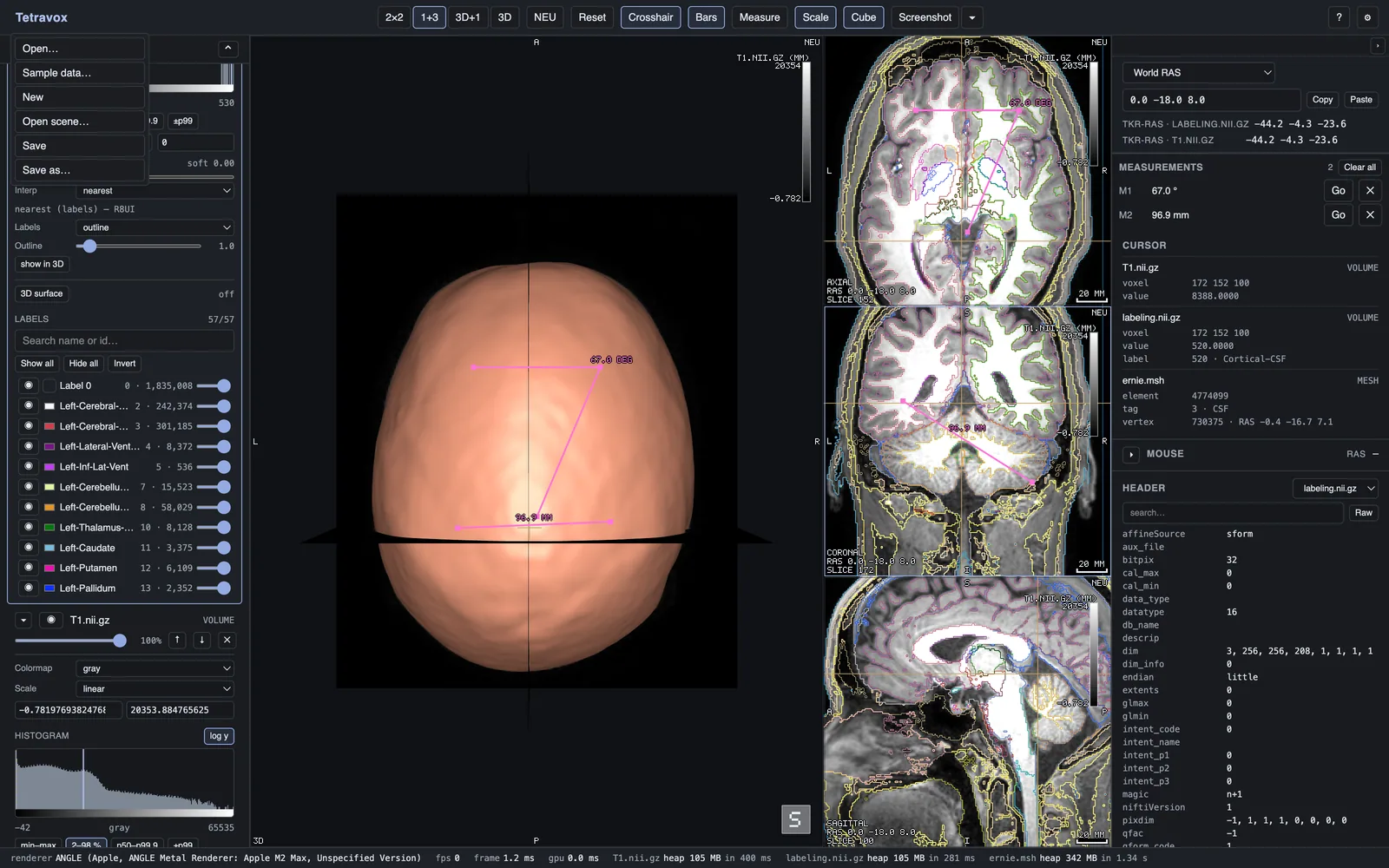
The app menu
Open, New, Open scene, Save and Save as.
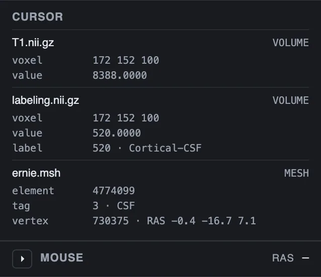
The cursor readout
Voxel, value and label under the cursor for every loaded dataset, volumes and mesh alike.
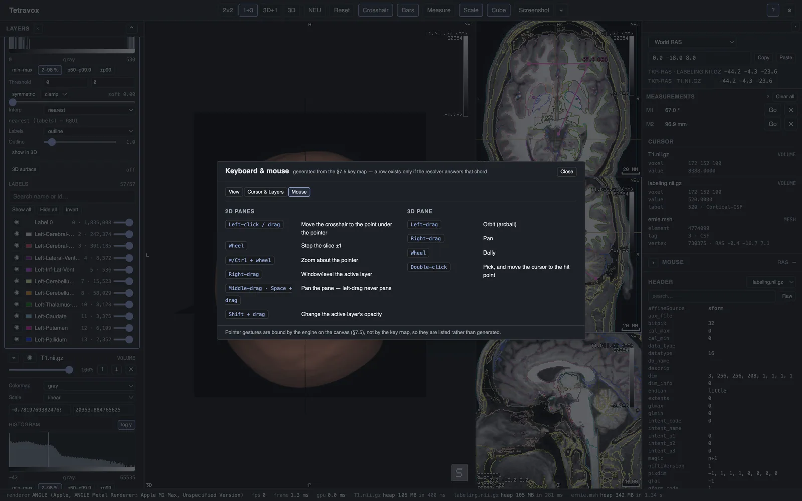
Keyboard & mouse — Mouse
The pointer gestures of the 2D panes and the 3D pane, listed rather than generated.
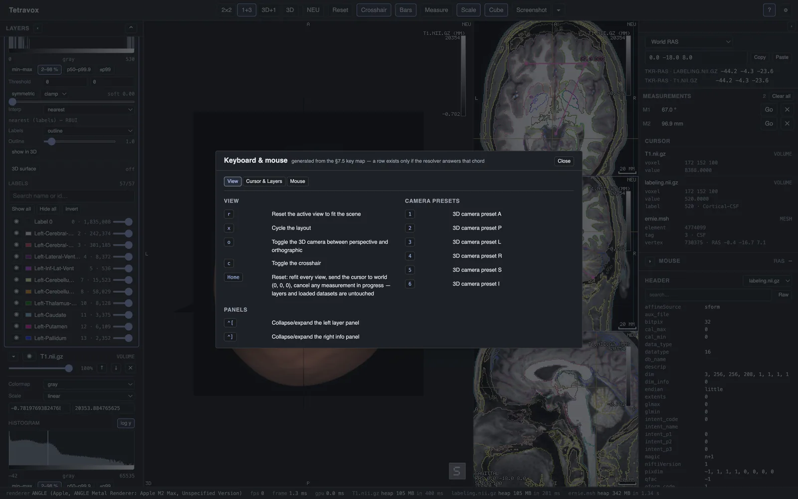
Keyboard & mouse — View
The tabbed key map generated from the key resolver: the View tab with camera presets and panel chords.
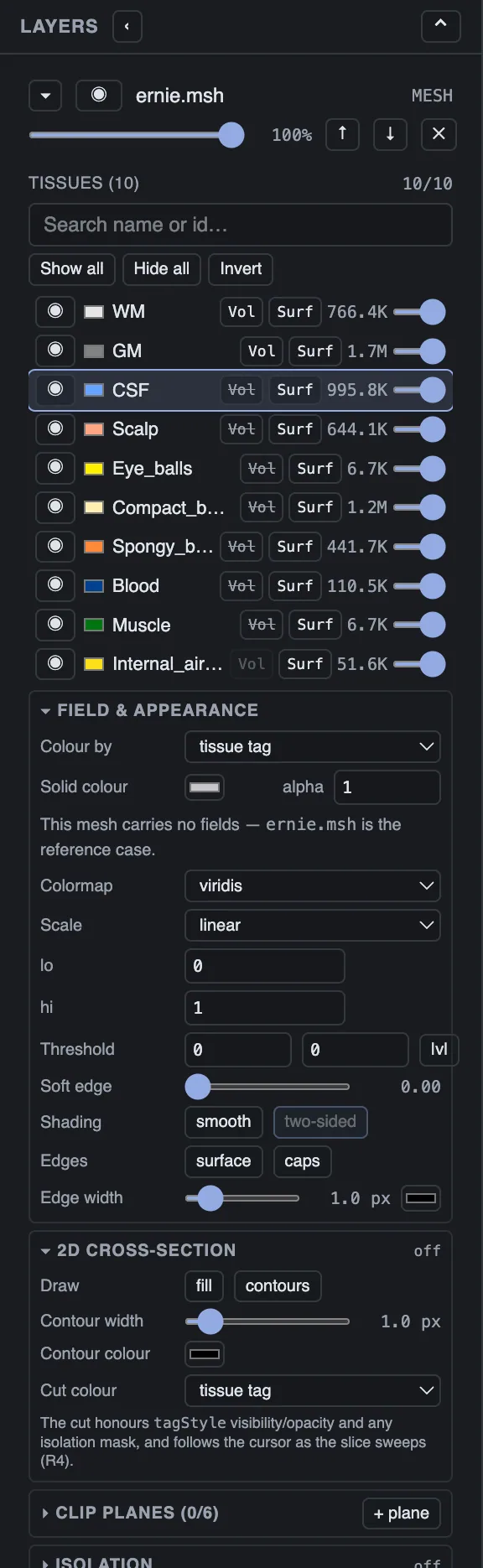
The layer panel
A mesh layer expanded: its tissue table, colour source, shading, edges and the 2D cross-section controls.
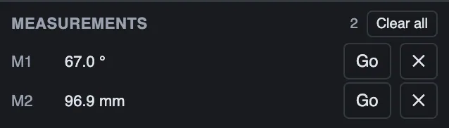
The measurement panel
Two measurements with their values, a Go button each, and Clear all.
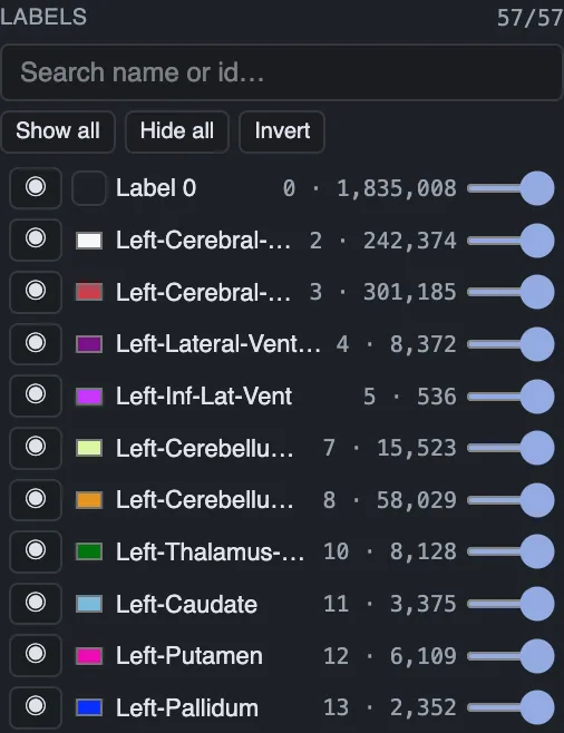
The region list
All 57 atlas regions, named from the LUT, each with visibility and opacity.
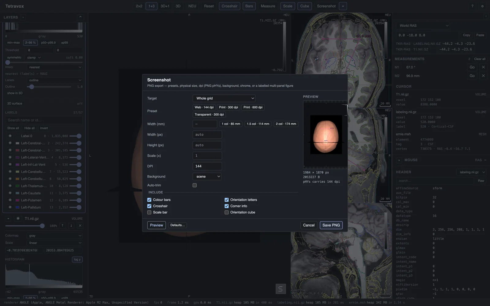
The screenshot export dialog
Target, dpi presets, physical width in millimetres, background, auto-trim and the per-capture chrome toggles, with a rendered preview and its byte size.
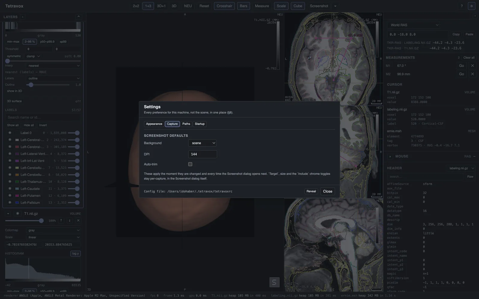
Settings — Capture
The screenshot defaults kept per machine: background, DPI and auto-trim.
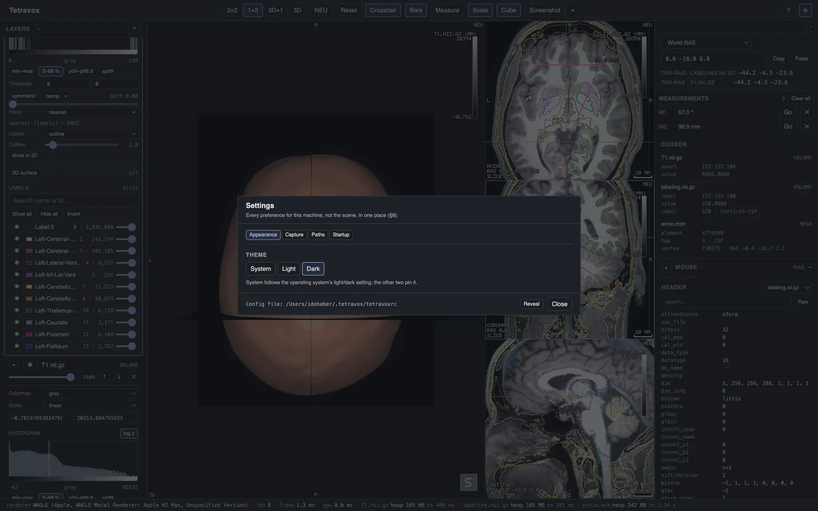
Settings — Appearance
The Settings dialog: tabs for Appearance, Capture, Paths and Startup, with the theme choice and the config file path.

The toolbar rail
Layouts, convention, reset, the annotation toggles, Measure and the Screenshot export menu.
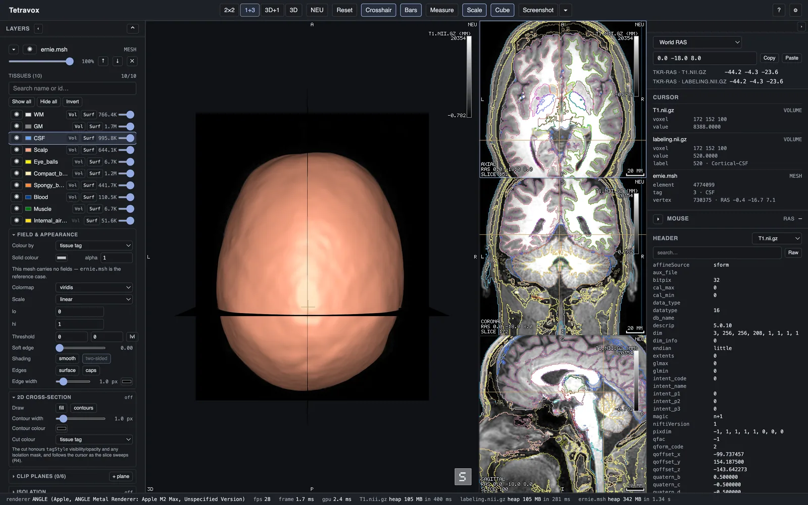
The window, dark
The whole application at 1600x1000 in the 1+3 layout: toolbar rail, layer panel with the mesh's tissue table, the info panel, the status bar.