Blener Integration

The Blender extension was built to enable publication level visualization and presentation of simulation results using other 3D modeling software in general, and specifically Blender. It provides a convenient interface for exporting cortical surfaces, field vectors, electrode placements, skin surfaces, and sub-cortical structures in formats compatible with Blender, CAD software, and other 3D visualization tools. Use it when you want a guided workflow from the GUI, or call the underlying Python scripts directly for batch jobs and automation.

Overview

• Location: tit/gui/extensions/visual_exporter.py
• Purpose: Export 3D assets in formats compatible with Blender, CAD software, and other 3D modeling tools to enable better visualization and presentation of simulation results.
• Back-end scripts:
  • blender/cortical_regions_to_ply.py
  • blender/cortical_regions_to_stl.py
  • blender/vector_ply.py
  • blender/electrode_placement.py
  • tools/extract_labels.py
  • tools/nifti_to_mesh.py
• Outputs: PLY surface meshes, STL geometry, PLY vector clouds, electrode placements (.blend/.glb), skin surfaces, and sub-cortical structures stored under the TI-Toolbox derivatives tree.

Supported Modes

Cortical Regions

This mode exports cortical surface regions defined by anatomical atlases as 3D mesh files. The exporter uses the central cortical surface mesh generated from your simulation and segments it according to the selected atlas labels.

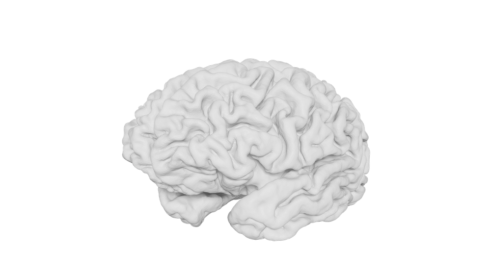
STL format export showing cortical surface geometry

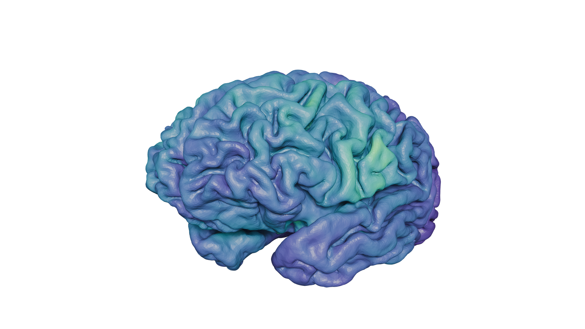
PLY format export with color-mapped field data

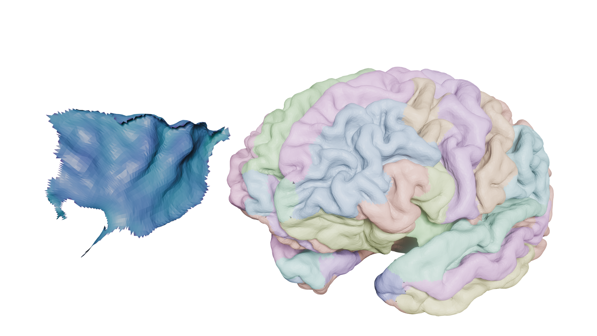
PLY format export showing detailed cortical regions

❮ ❯

What is produced:

• STL files: Binary STL format containing only geometry (no color information). These are lightweight files suitable for CAD software, 3D printing, or any workflow that doesn’t require color mapping.
• PLY files: PLY format with embedded color information. Each region is color-mapped according to the field values (e.g., TI_max) from the simulation mesh. These files preserve both geometry and field data for visualization in Blender or other 3D tools.

Atlas options:

• Choose from available atlases (DK40, DKTatlas40, HCP_MMP1, aparc.a2009s) based on your analysis needs.
• Select individual cortical regions to export, or export the entire atlas.
• Optionally include the whole gray matter (GM) surface as a single mesh file.

Output structure:

• Individual region meshes are stored in regions/ subdirectories.
• Whole GM surface is exported as a separate file when enabled.
• Optionally keep intermediate .msh files for audit trails and debugging.

Field Vectors

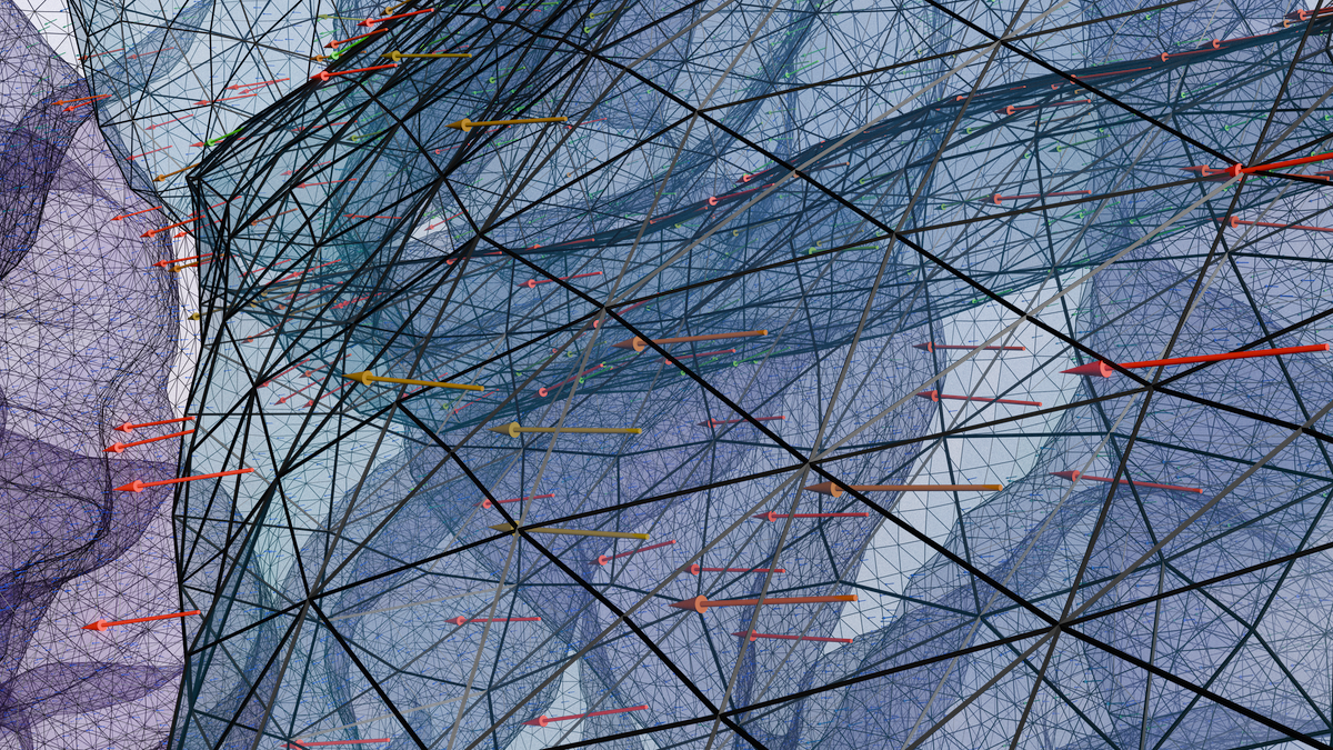
This mode exports electric field vectors from TDCS simulations as arrow clouds in PLY format. The vectors represent the electric field direction and magnitude at sampled points in the brain.

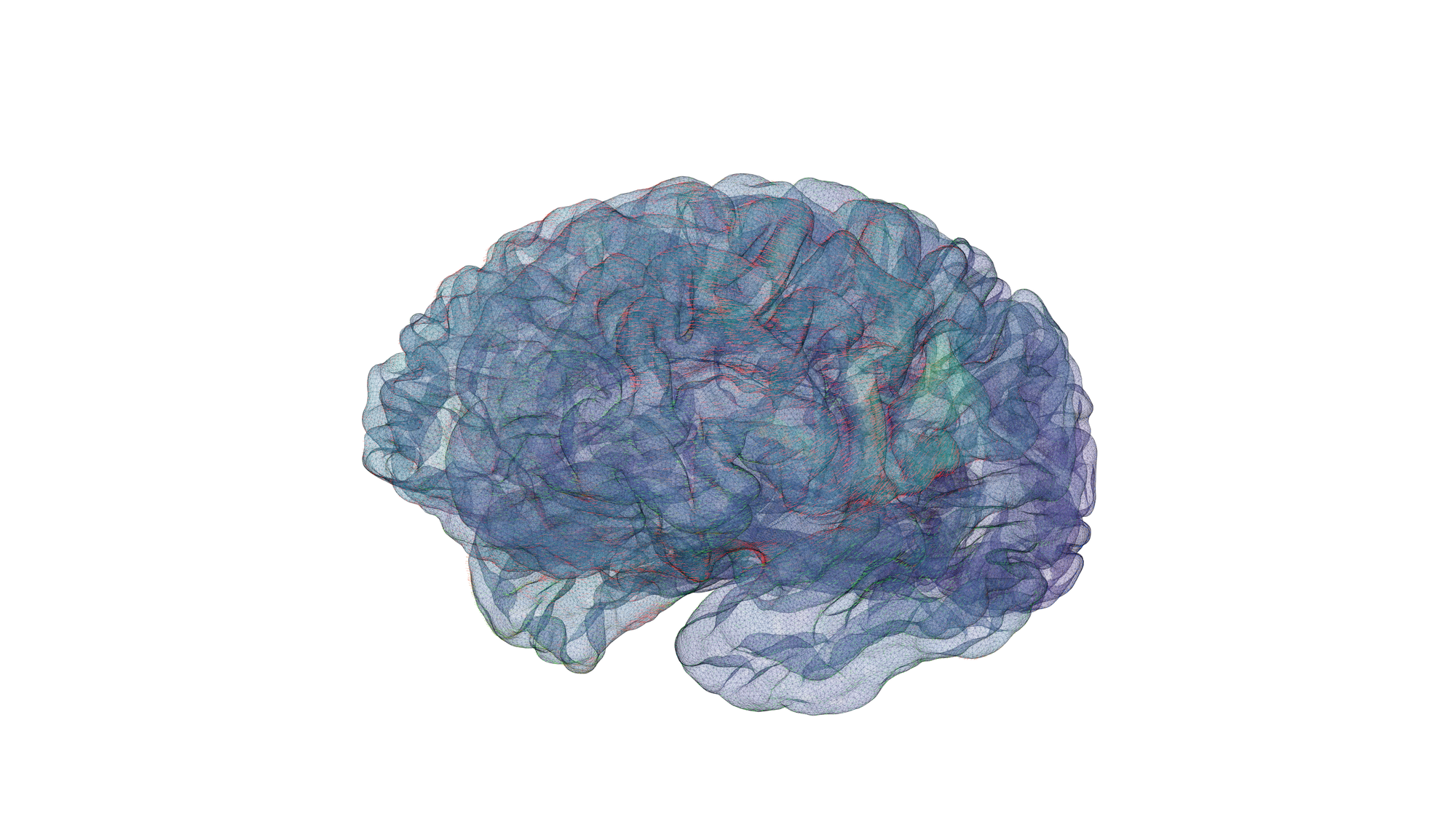
TI vector field visualization showing electric field directions and magnitudes

Close-up view of the vector field, highlighting individual arrow placement and detail

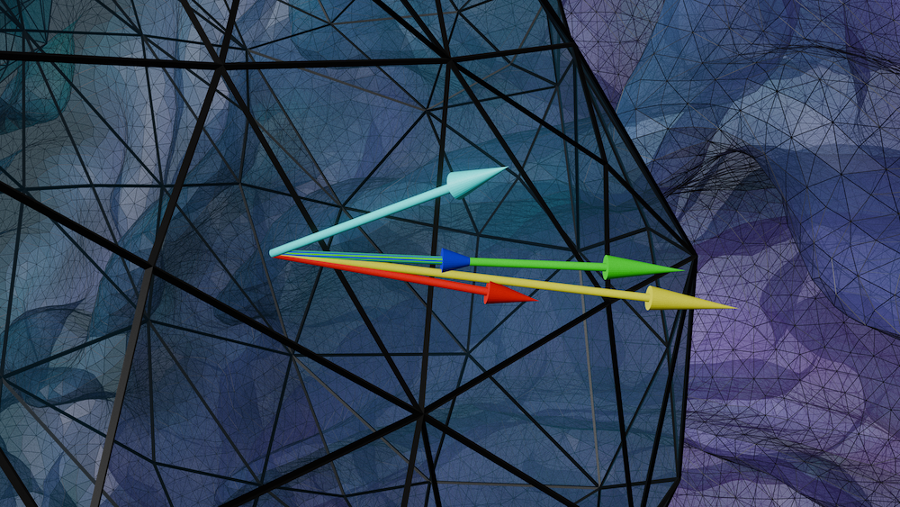
RGB color-coded vectors showing CH1 (red), CH2 (blue), TI (green), TI_sum (yellow), and TI_normal (cyan) fields

❮ ❯

What is produced:

• CH1 (Channel 1): Vector field from the first TDCS electrode configuration. Represents the electric field distribution (E1) when current flows through channel 1. Color: Red (RGB: 255, 0, 0) in RGB mode.
• CH2 (Channel 2): Vector field from the second TDCS electrode configuration. Represents the electric field distribution (E2) when current flows through channel 2. Color: Blue (RGB: 0, 0, 255) in RGB mode.
• TI (Temporal Interference): Modulation amplitude vectors representing the temporal interference pattern when two electric fields with slightly different frequencies interfere. The TI vector indicates both the spatial direction of maximum envelope modulation and the magnitude of maximum envelope amplitude (2 × effective amplitude). Calculated using the Grossman et al. 2017 algorithm, which computes the modulation amplitude when two sinusoidal fields E1(t) and E2(t) create a beating pattern. Color: Green (RGB: 0, 255, 0) in RGB mode.
• TI_sum: Optional output representing the vector addition of CH1 and CH2 (E1 + E2). This is the direct vector sum of the two electric field vectors, useful for visualizing the combined field distribution. Color: Yellow (RGB: 255, 255, 0) in RGB mode.
• TI_normal: Optional output representing the component of the TI vector normal to the cortical surface. This is particularly useful for understanding stimulation perpendicular to the cortex, as it isolates the component of the modulation amplitude that is orthogonal to the gray matter surface. Color: Cyan (RGB: 0, 255, 255) in RGB mode.

Vector properties:

• Each arrow’s direction represents the electric field direction at that point.
• Arrow length is scaled by the field magnitude (configurable via length scale parameter).
• Colors can be mapped using RGB mode (fixed colors per vector type: CH1=red, CH2=blue, TI=green, TI_sum=yellow, TI_normal=cyan) or magnitude-based scaling (magscale) to visualize field intensity across a blue-green-red gradient.
• Vector width and anchor point (tail or head) are customizable for visualization clarity.

TI vs mTI modes:

• TI mode: Uses 2 TDCS meshes (CH1 and CH2) to compute standard TI vectors.
• mTI mode: Uses 4 TDCS meshes (CH1, CH2, CH3, CH4) to compute multi-channel TI vectors, enabling more complex stimulation patterns.

Sampling options:

• Configure the number of vectors to sample (default: 100,000) or use all nodes for maximum detail.
• When using the maximum sample count, the script will produce a vector on every node of the given surface mesh. This is an expensive process that requires a large amount of memory and can take multiple hours for all vectors to be produced.
• Random seed controls reproducibility of sampling patterns.
• Vectors can be filtered to show only top percentile regions by magnitude.

Montage Visualizer

This mode creates 3D electrode placements on the scalp surface using Blender for visualization. It automatically extracts the scalp surface from the subject’s mesh file and places electrode objects according to EEG montage coordinates, with optional text labels.

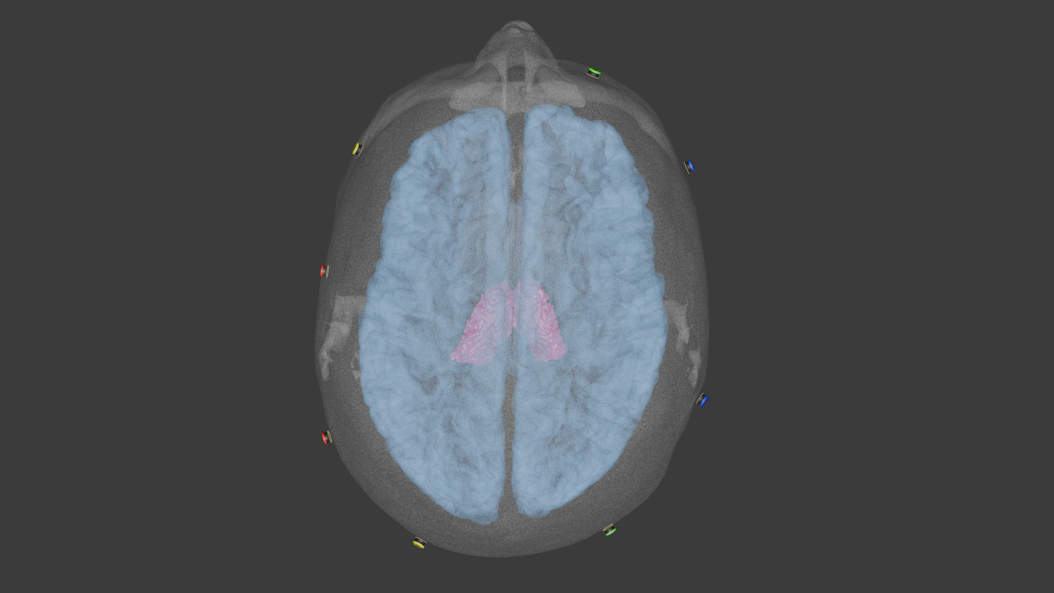
Electrode placement on scalp surface with sub-cortical thalamus ROI visualization

What is produced:

• .blend file: Blender scene file containing scalp surface, electrode objects, and text labels with sensible cameras, lighting conditions and material transparency.
• .glb file: GLTF binary format for web-based 3D viewers or other applications (e.g., electrodes_GSN-HydroCel-185.glb)
• scalp.stl: Extracted scalp surface mesh for reference

Electrode configuration:

• Choose from available simulation montages (automatically detected from the subject’s directory)
• Adjust electrode size, offset distance from scalp surface, and text label positioning
• Scale factor for coordinate system adjustments

Sub-cortical Extraction

This mode extracts sub-cortical structures from NIfTI segmentation files and converts them to 3D mesh formats. It can extract specific anatomical regions by label or export the entire segmentation volume.

What is produced:

• STL files: Binary STL format geometry files suitable for CAD software and 3D printing
• MSH files: SimNIBS mesh format for compatibility with simulation workflows
• NIfTI files: Copied segmentation files for reference

Segmentation options:

• Extract specific anatomical labels (e.g., thalamus: 10,49) or export the entire volume
• Optional cleaning of small disconnected components to reduce mesh complexity
• Automatic label extraction from FreeSurfer or other segmentation atlases

Input sources:

• Default: m2m_<subject>/segmentation/labeling.nii.gz (FreeSurfer segmentation)
• Custom: Any NIfTI file containing labeled anatomical regions

This can be incoporated into other visualization to produce images and animations such as:

Running from the GUI

1. Launch TI-Toolbox and click the Extensions button in the top-right corner of the window.
2. Select 3D Visual Exporter and click Launch.
3. Pick a subject and simulation from the dropdowns.
4. Choose Cortical Regions, Field Vectors, Montage Visualizer, or Sub-cortical mode.
5. Configure atlas, region filters, formats, and output directory options (for regions), sampling and styling parameters (for vectors), EEG montage and electrode settings (for electrode placement), or NIfTI file and label extraction settings (for sub-cortical structures).
6. Click Run Export. The console panel shows the exact commands executed and live progress.
7. Review artifacts in derivatives/ti-toolbox/visual_exports/sub-<id>/ once the export completes.

The Stop button terminates the active subprocess if you need to cancel a long export.

Running the scripts individually

You can call the Python scripts directly whenever you need command-line automation or custom batching. From within the TI-Toolbox environment, run:

# Export atlas-aligned cortical regions to PLY
simnibs_python blender_exporter/cortical_regions_to_ply.py \
  --mesh <path/to/central.msh> \
  --m2m <path/to/m2m_subject> \
  --output-dir <output_folder>

# Export region geometry to STL
simnibs_python blender_exporter/cortical_regions_to_stl.py \
  --mesh <path/to/central.msh> \
  --m2m <path/to/m2m_subject> \
  --output-dir <output_folder>

# Export TI or mTI vector arrows
simnibs_python blender_exporter/vector_ply.py \
  tdcs1.msh tdcs2.msh <output_prefix> --sum --ti-normal

# Place electrodes on scalp surface
simnibs_python blender_exporter/electrode_placement.py \
  --subject-id <subject_id> \
  --electrode-csv <path/to/eeg_positions/montage.csv> \
  --subject-msh <path/to/m2m_subject/subject.msh> \
  --output-dir <output_directory>

# Extract sub-cortical structures from NIfTI
simnibs_python tools/extract_labels.py \
  <path/to/labeling.nii.gz> \
  --labels 10 49 \
  --output <temp_extracted.nii.gz>

simnibs_python tools/nifti_to_mesh.py \
  <temp_extracted.nii.gz> \
  <output_mesh.stl> \
  --clean-components

Tips and troubleshooting

• Environment: Run the commands from within the TI-Toolbox environment. The scripts handle SimNIBS dependencies automatically.
• Missing fields: The cortical exporters expect the requested --field (default TI_max) to exist on the mesh. Inspect field names with simnibs_python -c "import simnibs; print(simnibs.read_msh('mesh.msh').field.keys())".
• Large vector clouds: Start with smaller --count values or enable --top-percent to reduce file sizes before ramping up density.
• Atlas updates: If you add a new atlas, ensure the m2m_* directory contains the matching label files before launching the GUI.
• Label extraction: When extracting specific labels, use comma-separated values (e.g., “10,49” for left/right thalamus). Check FreeSurfer’s label lookup table for anatomical region codes.
• Error logs: The extension console mirrors stdout/stderr from the scripts. Copy the failing command and re-run in a terminal to investigate with additional flags (for example --verbose).

Blender Tutorial: Visualizing PLY Files

This tutorial walks you through importing and visualizing PLY files exported from TI-Toolbox in Blender, including how to display the embedded color attributes.

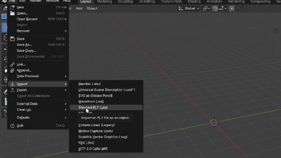
Step 1: Importing PLY Files

1. Open Blender and start with the default scene (or create a new project).
2. Go to File → Import → Stanford (.ply).
3. Navigate to your exported PLY file location (typically in derivatives/ti-toolbox/visual_exports/sub-<id>/<simulation>/ply/).
4. Select your PLY file and click Import Stanford (.ply).

The mesh will appear in your viewport. If the mesh appears very small or very large, you may need to adjust the view or scale the object.

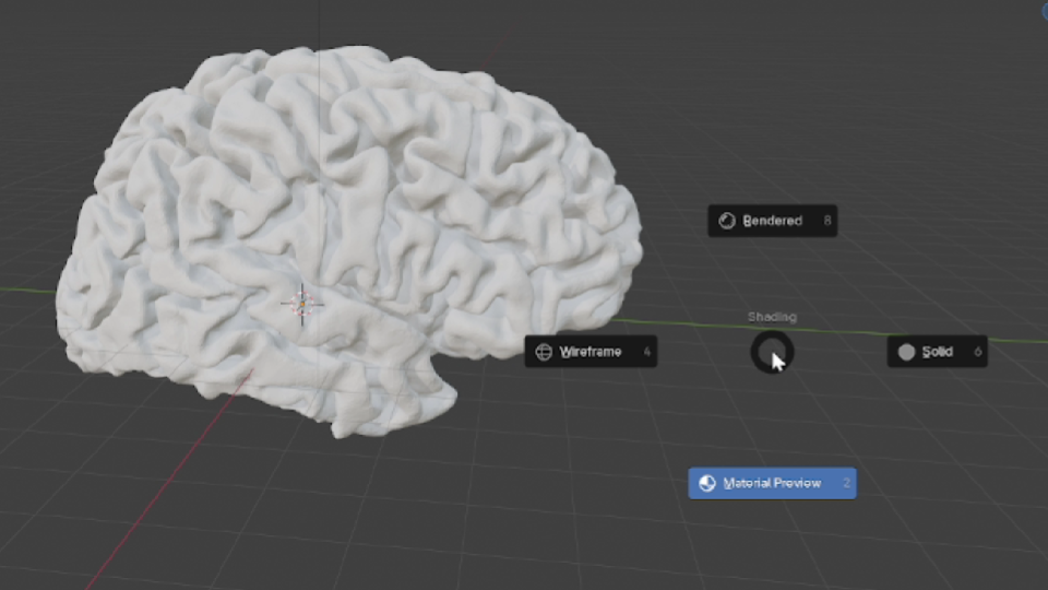
Step 2: Switching to Material Preview

To see materials and colors properly, switch the viewport shading mode:

1. In the 3D viewport, locate the viewport shading buttons in the top-right corner (or press Z to open the viewport shading menu).
2. Select Material Preview mode (or press Z then 2).

Material Preview mode provides a quick preview of how materials will look with basic lighting, making it ideal for checking color attributes.

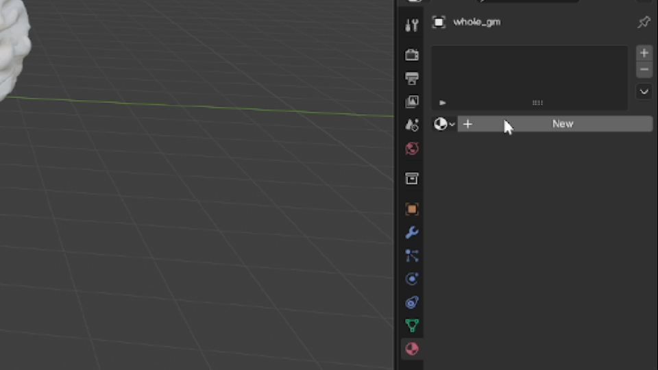
Step 3: Adding a Material

To display the color attributes from your PLY file, you need to create and assign a material:

1. Select your imported PLY mesh object in the viewport.
2. In the Material Properties panel (right sidebar, indicated by a sphere icon), click New to create a new material.
3. The material will be automatically assigned to your selected object.

Step 4: Setting Color to ‘col’ Attribute

To use the color data embedded in your PLY file (stored in the col attribute), set it as the material’s base color:

1. With your object still selected, in the Material Properties panel, locate the Base Color field (under the Surface section).
2. Click on the Base Color field.
3. Select Color Attribute from the dropdown menu.
4. In the attribute name field that appears, enter col (this matches the color attribute name in your PLY file).

Your mesh should now display the color-mapped field data from your simulation. The colors represent the field values (e.g., TI_max) that were exported with the mesh.

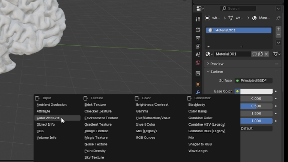
Adding the Attribute node and setting it to 'col'

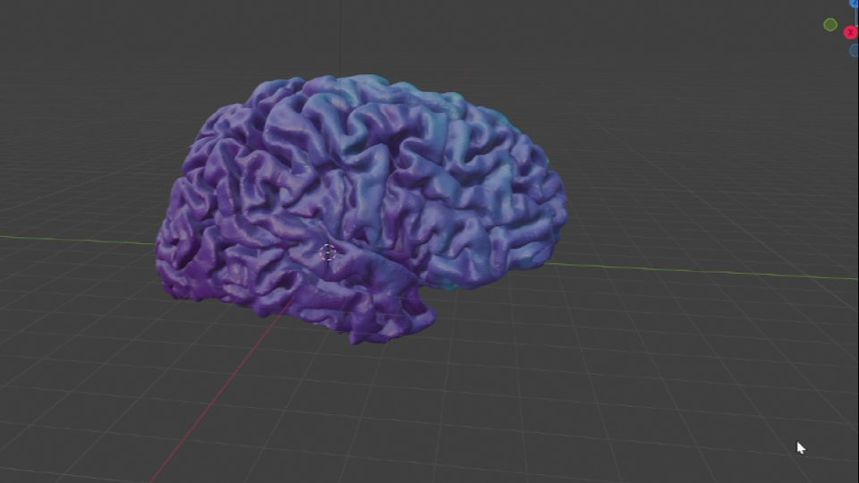
Final result with color attribute connected to the material

❮ ❯

Note: If your PLY file uses a different attribute name for colors, replace col in step 4 with the appropriate attribute name. You can check available attributes by selecting the mesh and viewing the Geometry Nodes or Mesh Data properties.